
What Is Compare Dates In Google Sheets?
Compare Dates in Google Sheets enables users to compare valid date values using basic operators such as =, <>, >, <, whether they are equal or not, greater than or less than, or to check the latest date. The operation returns the logical TRUE or FALSE results.
The Google Sheets Compare Dates finds it application while reviewing the sales data from different periods, tracking project progress in various phases, deriving age using birth dates, calculating EMI dates, etc.
For example, we have the same date in two valid formats as short date and long date. Let us check if the valid date values are equal or not.

Select cell C1, enter the formula =A2=B2 and press “Enter”, as shown below.

The output is shown above. Both the date values are same, except that they are in different formats. Hence the result is TRUE, indicating that the values are same.
Use this Compare Dates In Google Sheets Template to follow along with the examples in this article.
Download Excel TemplateKey Takeaways
• The Compare Dates in Google Sheets enables us to check if the selected dates with a valid format are the same or not, is one value greater than the other or not.
• Entering date as cell references rather than as cell values are advisable to get correct results.
• We can use logical operators, ‘=’, ‘>’, ‘<’, ‘>=’, ‘<=’, and ‘<>’, to compare date values in a worksheet.
• The results are always the logical TRUE or FALSE. Therefore, the IF function plays a dominant role when combined with the comparison equation to get an alternate or better interpretable results.
• We can use the DATE() or TODAY() functions for date arguments inputs to avoid errors.
How To Compare Dates In Google Sheets?
We can compare dates in Google Sheets using the following methods, namely,
- Check if Dates are Equal.
- Check if Dates are Not Equal.
- Check if First Date is Greater than Second Date.
- Check if First Date is Less than Second Date.
- Find Which Date is Latest.
Method #1 – Check if Dates are Equal –
Step 1: In an empty cell, insertequal sign, i.e., “=”, to start the equation andenter value1 as a cell value or a cell reference.
Step 2: Next, insert the equal sign, i.e., “=”, then, enter value2 as a cell value or a cell reference and press “Enter”.
The syntax will then be “=value1=value2”
Method #2 – Check if Dates are Not Equal
Step 1: In an empty cell, insertequal sign, i.e., “=”, to start the equation andenter value1 as a cell value or a cell reference.
Step 2: Next, insert the not equal sign, i.e., “<>”, then, enter value2 as a cell value or a cell reference and press “Enter”.
The syntax will then be “=value1<>value2”
Method #3 – Check if First Date is Greater than Second Date
Step 1: In an empty cell, insertequal sign, i.e., “=”, to start the equation andenter value1, or first date,as a cell value or a cell reference.
Step 2: Next, insert the greater than sign, i.e., “>”, then, enter value2, or second date,as a cell value or a cell reference and press “Enter”.
The syntax will then be “=value1>value2”
Method #4 – Check if First Date is Less than Second Date
Step 1: In an empty cell, insertequal sign, i.e., “=”, to start the equation andenter value1, or first date,as a cell value or a cell reference.
Step 2: Next, insert the less than sign, i.e., “<”, then, enter value2, or second date,as a cell value or a cell reference and press “Enter”.
The syntax will then be “=value1<value2”
Method #5 – Find Which Date is Latest
We must use the IFS() function to Find Which Date is Latest and the syntax is,
=IFS(value1>value2, “First Date”, value1<value2, “Second Date”, value1=value2, “Equal”).
Examples
Let us consider some Compare Dates in Google Sheets examples to understand the above-mentioned methods we learnt.
Example #1 – Dates are equal or not
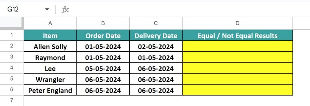
The table below consists a few shirt brands, their order and delivery dates. We will compare the dates and check if the Dates are equal or not.
The steps to compare if the Dates are equal or not are,
Step 1: Select cell D1 and enter the formula =B2=C2, as shown below.

Step 2: Press “Enter”. Here, Google Sheets provides and autofill option, either select that or use the fill handle method.

Step 3: Drag the formula from cell D2 to D6 using the fill handle, to get the following results.

The output shown above indicates that rows 3, 5 and 6 date values are equal and hence TRUE, and rows 2 and 4 date values are not equal and hence FALSE.
Example #2 – Dates are greater than or less than
Consider the dataset that consists of Project details, such as their names, the deadline date for all the projects and the date they were submitted. We will compare the dates and check if the Dates are greater than or less than the submission date.

The steps to compare if the Dates are greater than or less than the submission dateare,
Step 1: Select cell D1 and enter the formula =”10-05-2024″>C2, as shown below.

Step 2: Press “Enter” and drag the formula from cell D2 to D7 using the fill handle, to get the following results.

[Note: Alternatively, if we would have entered the formula as =”10-05-2024″<C2 in cell D2, then the results will be exact opposite from what has resulted now, i.e., TRUE will become FALSE and vice versa, because of the less than symbol.]
Step 3: We can also insert the IF() function to get alternate results instead of the default TRUE or FALSE. Let us try that as well.
Therefore, select cell E2, enter the formula =IF((“10-05-2024″>C2)=True,”Greater”,”Less”), press “Enter” and drag the formula from cell E2 to E7 using the fill handle, to get the following results.

Example #3 – Compare Dates with different formats
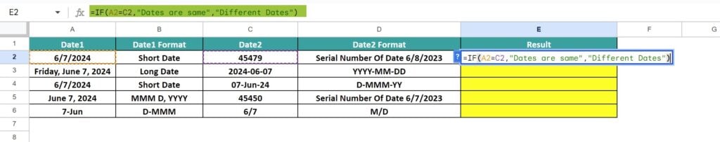
We have a single date written in various available valid formats in the dataset given below. Columns A and C are the same date, except for one different date, entered in different formats and Columns B and D provides the entered date format details, respectively. Let us Compare Dates with different formats and get alternate results using the IF function.

The steps to Compare Dates with different formats along with the IF function are,
Step 1: Select cell E2 and enter the formula =IF(A2=C2,”Dates are same”,”Different Dates”), as shown below.
Step 2: Press “Enter” and drag the formula from cell E2 to E6 using the fill handle, to get the following results.

The output is shown above.
- The cells in rows 3 to 6 of columns A and C contain the same date value, 6/7/2023, in different formats. Since, it satisfies the condition, the IF() formula returns the result “Dates are same”.
- However, in row 2, cell C2 contains a preset date serial number, but not of the compared date. Therefore, the IF() condition is not fulfilled, hence the result is “Different Dates”.
Example #4 – Check the latest date
The dataset consists same date in column A, as first dates and different dates in column B, as second dates. We will compare the dates to Check the latest date using the IFS function in Google Sheets and get the results of the fulfilled condition.

The procedure to Check the latest date using the IFS function are,
Select cell C2, enter the formula =IFS(A2>B2,”First Date”,A2<B2,”Second Date”,A2=B2, “Equal”), press “Enter” and drag the formula from cell C2 to C3 using the fill handle, to get the following results.

The output indicates that in the first set of dates the first date is the latest and in the next row, i.e. the second set of dates the second date is the latest.
Important Things To Note
- When we enter formulas to Compare Dates in Google Sheets, the program considers the sequential serial number equivalent of each date value for calculations.
- Sometimes a text may appear like a date value. So, before comparing dates, confirm the supplied values are in the required date format to avoid the formula returning errors or incorrect values.
Frequently Asked Questions (FAQs)
A few reasons why the Compare Dates in Google Sheets may not work are,
• The entered dates are invalid date values or invalid formats.
• We have not used the right operator or symbol while comparing the dates.
• The date value directly entered as a cell value is not enclosed within double-quotes.
• The date format is changed to text when we copy-paste data.
We can insert the IF() function in Google Sheets as follows:
Choose an empty cell for output – select the “Insert” tab – click the “Function” option right arrow – click the “Logical” option right arrow – select the “IF” function, as shown below.
The IF formula appears as shown below. 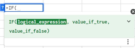
Sometimes we cannot remember in which category the “IF” function falls. Then, we can insert the function as follows:
Choose an empty cell – select the “Insert” tab – click the “Function” option right arrow – click the “All” option right arrow – select the “IF” function, as shown below.
However, as always, entering the function manually is the best way to avoid confusion.
[Note: Alternatively, we can also find the function icon to insert the IF function by following the path shown below.
Choose an empty cell – click the “More” option represented by the three vertical dots at the end of the toolbar, as shown below.
A list of icons appears when we click the “More” option. Here, click the “Functions” icon, as shown below.
When we click the “Functions” icon, we get the details shown in the below image.
From here, we know the rest to select the required function.
Use this Compare Dates In Google Sheets Template to follow along with the examples in this article.
Download Excel Template