FV in Google Sheets

What Is FV in Google Sheets?

The FV in Google Sheets stands for ‘Future Value’. It basically calculates the future value of investments with compound interest. The arguments required to use the FV formula include the knowledge of periodic payments (these can be annual, quarterly, weekly, etc.) and a fixed interest rate. Future value helps in financial planning by helping you understand the growth of an investment. At the same time, it is easy to calculate FV when the rate of interest is fixed, such as in a savings account; it can be difficult for bonds, etc. due to a volatile rate of return.

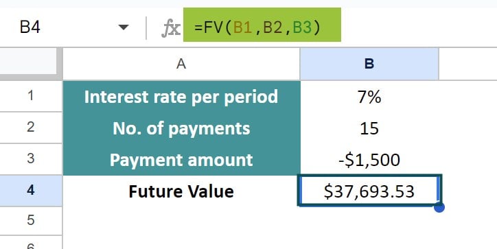
FV in Google Sheets works for a single lump sum or periodic payments. Below, you can see a simple way to implement the formula. Let’s suppose you make a yearly payment of $1,500 for 15 years with an annual interest rate of 7%. All payments are made at the year’s end and are considered a regular annuity. To find the future value, enter the following formula:

=FV(B2, B3, B4). Here, the payment is negative as it is a cash outflow.

FV() Google Sheets Formula

The FV in Google sheets can be calculated using the following formula.

=FV(rate, number_of_periods, payment_amount, [present_value], [end_or_beginning])

Here,

1. rate: the fixed rate of interest over time. If it is monthly, the value is divided by 12; if quarterly, by 4, and so on.
2. number_of_periods: the number of periodic payments to be made
3. payment_amount: the amount of money that you pay for each period.
   • It may be weekly (52), monthly (12), or quarterly (4) multiplied by the time period. For example, a monthly payment made for a period of 5 years will be 12*5 = 60 periods.
4. [present_value]: (optional value, 0 by default) the current value of the investment.
5. [end_or_beginning]: [optional,  0 by default] 0 indicates that you are making the payments at the end of each period, while 1 indicates payment made at the beginning.

How to calculate future value in google sheets?

From the Google Menu

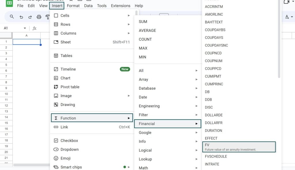
You can easily insert the FV function from the Google Sheets menu.

First, go to the “Insert” option. Go to “Functions” and choose “Financial.” Choose the FV function and enter the required arguments.

Manually Entering the FV function

In addition to the Google menu, you can also enter the FV directly in Google Sheets with the necessary arguments, such as the rate of interest, the payment period, and the amount to be invested.

 Let us say you invest $5,000 for two years and receive a rate of interest of 6%. Find the future value of this investment at the end of two years.

Step 1: Enter the given details in a Google sheet.

The amount of $5,000 is entered as the payment amount and since it is an outflow, we enter it as a negative value.

Step 2: To find the FV in Google Sheets, enter the following function in cell B4.

=FV(B1, B2, 0, B3, 0)

This is based on the formula =FV(rate, number_of_periods, payment_amount, [present_value], [end_or_beginning]).

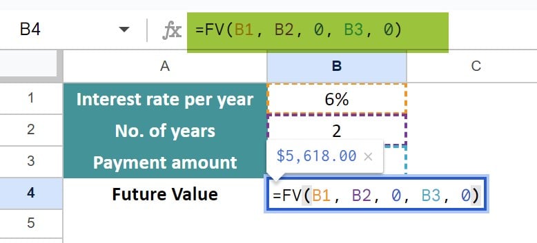
Here, as there are no intervening payments, the payment amount is taken at 0 in argument 3. Now, press Enter to get the future value in cell B4.

We use zero as the payment argument since there are no intervening payments. The future value is calculated as $5,618.00 after a period of two years.

Examples

You can effectively use FV in Google Sheets as a financial function to calculate the future value. Let us look at some examples of how to calculate future values under different everyday scenarios.

Example #1 – Calculate the future value of a lump-sum payment

You can also calculate the future value in Google Sheets when you make a one-time investment payment over some time. For example, you may choose to invest a lump sum one time in a new venture. Here, the future value will be based on the present value rather than the periodic payment.

Let’s say we have invested $100,000 as a lump sum over the next 10 years. The annual interest rate is 5%.

Step 1: Enter all the details in a Google sheet.

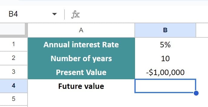
Step 2: As this is a lump sum going into the investment, it’s important to remember that the value is negative.

To calculate the future value of this lump-sum, input the following formula.

=FV(B1,B2, , B4)

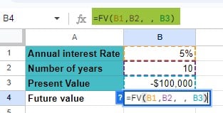
Step 3: Press Enter. As seen below, you will end up with $162,889.46 at the end of 10 years!

Example #2 – Calculate the future value of an investment

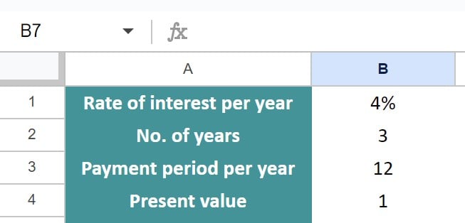
FV is applicable not just for loans but also in calculating the future value of an investment. Suppose a businessman has an account for business savings and deposits $10,000 every month into it over three years. The rate of interest annually is 4%. Let us calculate the FV at the end of three years. We make payments at the beginning of each month.

Step 1: As he is paying a monthly amount, the rate of interest is divided by 12, and the number of payments should be calculated by multiplying the period by 12.

For clarity, let us enter all the details in a Google Sheet.

Step 2: To calculate the future value of the investment after three years, input the following formula:

=FV(B1/B3, B2*B3, B5, 0, B4) in cell B6.

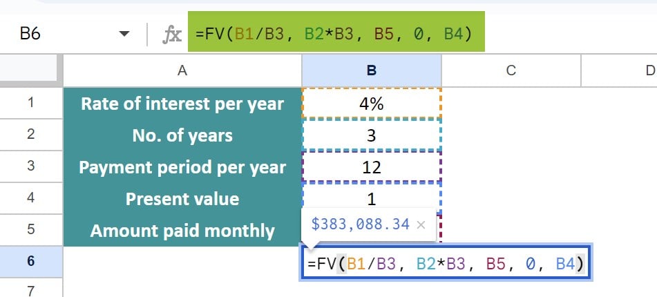
Step 3: Press Enter. The total investment over three years would be $383,088.34.  

Example #3 – Calculate loan payback

The FV formula is also helpful in calculating whether you will be able to pay off a loan in a particular amount of time. For this, you must calculate whether an investment over a certain period gives you a positive balance. If the result is positive, you will successfully pay back the loan in time else you have to increase the value of your payments or the number of payment duration.

A student has taken out a loan of $10000. He wants to pay it back over three years in $900 installments at the end of each quarter. The loan’s annual interest rate is 5%.

Step 1: To calculate the FV at the end of three years, input the following formula in cell  B6

=FV(B1/B3,B2*B3,B5,B4,0)

We are dividing the interest by 4 as it is an annula interest but our payment is quarterly. Similarly, for three years we are multiplying by 4 for quarterly payment.

Step 2: Press Enter.  

As shown in the image, the value returned is negative. This means that the amount we are paying back will not be complete in three years.

Step 3: You can alter the value slightly as a $1000 payment per quarter and check the result.

Thus, a slight alteration in the quarterly payment helps the student settle the loan in three years.

Important Things To Note

1. If you do not specify the payment amount(third argument), you should specify the present value and vice versa.
2. As the payment amount and present value represent outflows, we give them a negative sign.
3. You convert the annual interest rate to a periodic one based on the number of periods per year.
   • Semi-annual = interest rate/2
   • Quarterly = interest rate/4
   • Monthly = interest rate/12
4. Also, to get the total number of periods, multiply the years term with the number of periods per year
   • Semiannual payments: no. of years * 2
   • Monthly payments: no. of years * 12
   • Quarterly payments: no. of years * 4

Frequently Asked Questions (FAQs)

Download Template

This article must help understand the FV in Google Sheets, with its formula and examples. You can download the template here to use it instantly.

Recommended Articles

Guide to What Is FV in Google Sheets. We learn FV in Google Sheets, its examples, working template. You can learn more from the following articles.

Compound Interest In Google Sheets

PV in Google Sheets

Rate Function in Google Sheets