
What Is “Greater Than Or Equal To” (>=) In Google Sheets?
The “Greater Than or Equal To” (>=) in Google Sheets is a logical operator used for comparing two values of same data type. It returns TRUE if the first value is either bigger than or equal to the second value, else it returns FALSE. The Greater Than or Equal To symbol in Google Sheets is “>=” and is widely used to compare numeric values, dates, time and textual data.
For example, we have the textual data given below that consists of animal names. We will use the Google Sheets “Greater Than or Equal To” (>=), to compare the values.
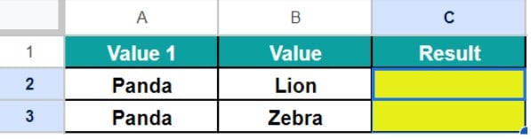
Select cell C2, enter the formula =A2>=B2, press “Enter” and drag the formula from cell C2 to C3 using the fill handle.

The output is shown above as per the universal rule where the values “A” and “Z” are considered the lowest and the highest text values, respectively.
- The cell C2 is TRUE, because the first letter “P” in Panda is greater than the letter “L” in Lion.
- The cell C3 is FALSE, because the first letter “P” in Panda is less than the letter “Z” in Zebra.
Use this “Greater Than Or Equal To” (>=) In Google Sheets Template to follow along with the examples in this article.
Download Excel TemplateKey Takeaways
- The logical operator, “Greater Than or Equal To” (>=) in Google Sheets, compares two values and returns TRUE if the first data is equal to or more than the second data. Otherwise, the operator returns FALSE.
- We can directly use the “Greater Than or Equal To” logical operator in a formula cell.
- The two values we compare using the “Greater Than or Equal To” logical operator should be of the same data type.
- We can apply the “>=” logical operator in the test conditions in functions such as, COUNTIF(), IF() and SUMIF(). Also, we can still compare values without the operator, using the Conditional Formatting “Greater than or equal” rule.
How To Use “Greater Than Or Equal To” (>=) In Google Sheets?
The steps To Use “Greater Than or Equal To” (>=) in Google Sheets are as follows:
Step 1: Ensure we have a minimum of two data values of same or different data type.
Step 2: First, select the result/target cell. Type the “equal to” (=) sign.
Step 3: Next, enter the first value or cell reference of the first value.
Step 4: Then, enter the following. Greater Than or Equal To sign in google sheets, i.e., “>=”.
Step 5: Next, enter the second value or a cell reference of the second value.
The syntax will be as shown below,

or

Step 6: Finally, press “Enter” to get the logical result.
Examples
Let us consider some “Greater Than or Equal To” (>=) in Google Sheets examples, along with other functions such IF(), SUMIF(), COUNTIF() and Conditional Formatting.
[Note: With these functions we can also get alternate results, instead of the default, TRUE or FALSE, logical results.]
Example #1 – “Greater Than or Equal To” with the IF Function.
Consider the data table below that consists of employee names and the units of a product they sold for a month. If the employees have sold more the 15,000 units, then they will get bonus for that particular month. We will use the “Greater Than or Equal To” with the IF Function to check if they are eligible for bonus or not.

The steps to use the “Greater Than or Equal To” with the IF Function are:
Step 1: Select cell C2 and enter the formula =IF(B2>=15000,“Bonus”,“No Bonus”)

Step 2: Press Enter to get the output, as shown below.
[Note: Google Sheets gives an Auto Fill suggestion, we can accept it or follow the fill handle method.]

Step 3: Drag the formula from cell C2 to C6 using the fill handle, to get the following eligibility results.

Example #2 – “Greater Than or Equal To” with the COUNTIF Function.
Consider the below table showing a list of products and the quantities ordered. We will use the “Greater Than or Equal To” with the COUNTIF Function to count the number of products that fulfills the given criteria.

The procedure to use the “Greater Than or Equal To” with the COUNTIF Function are:
Select cell D4, enter the formula =COUNTIF(A1:B11,”>=250″) and press “Enter”.

The output is 7, as shown above. We have highlighted the products that fulfill the given criteria, for our reference.
Example #3 – “Greater Than or Equal To” with the SUMIF Function.
The below table shows representative details with their sales for the year 2023-2024. We will use the
“Greater Than or Equal To” with the SUMIF Function to find the sum of the sales that fulfills the criteria or condition.

The procedure to use the “Greater Than or Equal To” with the SUMIF Function are:
Select cell B11, enter the formula =sumif(A1:B8,”>=30000″) and press “Enter”.

The total sales is “$200,000”, as shown above. We have highlighted the representative sales that fulfill the given criteria, for our reference.
Example #4 – “Greater Than or Equal To” in Conditional Formatting.
We have the following table that consists of some brands and their quarterly sales for the months of July to September. We will use the “Greater Than or Equal To” in Conditional Formatting to highlight the cell values that satisfy the criteria.

The steps to use the “Greater Than or Equal To” in Conditional Formatting are as follows:
Step 1: Choose the data range A2:D8 – select the “Format” tab – click the “Conditional formatting” option. When the “Conditional format rule” pane opens on the right, click the “Add another rule” option, as shown below.

Step 2: Now, select the “Single color” tab and under the “Format rules” section,
- First, click the “format if…” drop-down, select the “greater than or equal to” option and enter 50,000 in the “Value” field that appears as soon as we select one of the options from the drop-down.
- Next, in the “Formatting style” options, select the color “Pink” from the “Fill color” option.
- Finally, click the “Done” button, as shown below.

We get the output shown below. All the cells that is greater than or equal to $50,000 are highlighted.

Important Things To Note
- If the values are of different data type, then we get the answer as FALSE, when using the logical Greater Than or Equal To “>=” operator. Again, depending on the conditional function used, we may get a “#VALUE!” error.
- We must enter the argument values, either as cell values or cell references. Ensure to enter the direct values or conditions with values within double-quotes. If not, we will get an incorrect output.
Frequently Asked Questions (FAQs)
The COUNTIF function in Google Sheets is inserted as follows:
Choose an empty cell for the output – select the “Insert” tab – click the “Function” option right arrow – click the “Math” option right arrow – select the “COUNTIF” function, as shown below.
We can insert the COUNT functions such as, COUNTIF, COUNTIFS, COUNTBLANK, COUNTUNIQUE, etc. using the path shown above.
We will consider a couple of ways to clear conditional format for blank cells in google sheets.
If the output has multiple rules applied, as shown in the image below.
To clear the rules that are not required, just hover around the set rules and we will see a delete option. Click it, as shown below.
Then we will get the output, as shown below.
We can use the above learnt option to clear single or multiple rules at once.
However, if we must clear all the rules set for a dataset, such as formatting styles or conditional formatting, then, we can proceed with the following steps,
Select the entire worksheet or just the dataset – go to the “Format” tab – click the “Clear formatting” option, as shown below.
The “Greater Than or Equal To” >= in Google Sheets should be used in the following situations:
a. To find which of the two quantities is greater or smaller.
b. To find whether one quantity is equal to the other.
c. To evaluate two quantities with respect to a given criterion.
d. To compare two separate quantities with a third quantity.
We often forget in which category a function falls, here, the “SUMIF” function. Then, we can insert the function as follows:
Choose an empty cell – select the “Insert” tab – click the “Function” option right arrow – click the “All” option right arrow – select the “SUMIF” function, as shown below.
Use this “Greater Than Or Equal To” (>=) In Google Sheets Template to follow along with the examples in this article.
Download Excel Template