ANOVA In Excel

What Is ANOVA In Excel?

ANOVA or Analysis of Variance, is a statistical analysis that evaluates whether the mean values of two or more independent groups are significantly different or not. ANOVA In Excel assesses the impact of one or multiple factors by comparing different mean values. It helps users understand the variance of variables, and they can use it to perform null hypothesis testing and regression analysis.

For example, the following table contains the score details of three students.

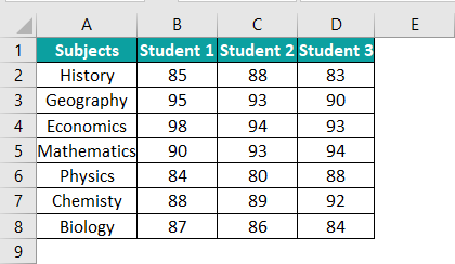
Using the single-factor ANOVA in Excel technique, we can examine if the mean values of the three datasets i.e., the scores of Students 1, 2, and 3, are the same or significantly different.

Now, we can see whether to accept or reject the null hypothesis if there is no significant difference in the mean values of Student 1, Student 2, and Student 3 scores.

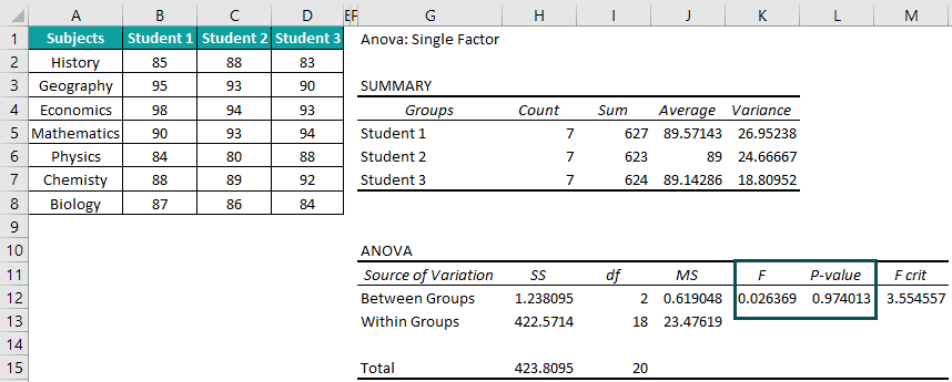
Once we calculate ANOVA in Excel, we get the output shown in the above image.

Output Observation: The F and p-value are the most critical parameters in an ANOVA in Excel. In the above example, the F value is less than the F crit value (F critical). Also, the p-value is more than Alpha, the significance threshold (typically 0.05). Thus, we cannot reject the null hypothesis, and the mean values of the three students’ scores are not significantly different.

What Is ANOVA In Excel?

ANOVA in Excel is a statistical method used to determine if the mean values of various groups in a model are significantly different or not.
Excel offers three types of ANOVA tests, single-factor, two-factor with replication, and two-factor without replication.
The Analysis Tools list in the Data Analysis window will show the ANOVA tests.
The F and p-value are the two most important parameters we need to check in the ANOVA test result. They decide whether to accept or eliminate the null hypothesis and determine which independent variables affect the dependent variable.

Where Is ANOVA In Excel?

Although the function exists, ANOVA in Excel is not enabled by default.

Initially, the “Data” tab will be as shown below.

Let us first enable the Excel add-in “Analysis ToolPak” so that we can calculate ANOVA in Excel.

The steps to enable the Analysis ToolPak add-in are:

Step 1: Choose File > Options to open the Excel Options window.

Step 2: Click the Add-ins option on the left in the Excel Options window. On the right side, below, check if the Manage field is Excel Add-ins, and click Go… to open the Add-ins window.

Step 3: In the Add-ins window, check/tick the “Analysis ToolPak” checkbox and click “OK”.

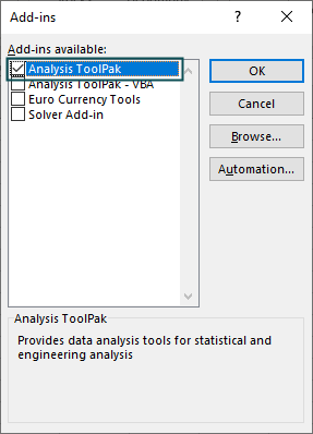
Once we click “OK”, the “Data” tab will show the “Data Analysis” option.

Now, select the “Data” tab > go to the “Analysis” group > click the “Data Analysis” option to open the “Data Analysis” window to access the ANOVA functions.

In the “Data Analysis” window, we see the ANOVA options in the “Analysis Tools” list.

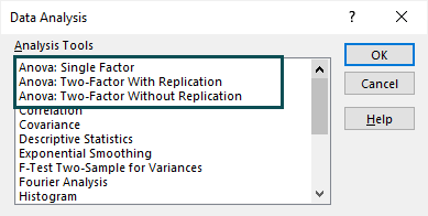
The first option will enable us to perform a one-way ANOVA test or single-factor ANOVA in Excel. We can conduct a two-way ANOVA test in Excel with the other two options.

Excel VBA – All in One Courses Bundle (35+ Hours of Video Tutorials)

If you want to learn Excel and VBA professionally, then Excel VBA All in One Courses Bundle (35+ hours) is the perfect solution. Whether you’re a beginner or an experienced user, this bundle covers it all – from Basic Excel to Advanced Excel, Macros, Power Query, and VBA.

Start Learning Now

One Way ANOVA Test In Excel

The one-way ANOVA test compares the mean values of datasets and determines if they are different. We will use the “ANOVA: Single Factor” option from the “Data Analysis” window.

The following table shows the tensile strength data collected during three tests.

The steps to conducting the One-Way ANOVA Test in Excel are:

1: Select the “Data” tab > go to the “Analysis” group > click the “Data Analysis” option.

2: Once the Data Analysis window opens, choose the first option i.e., “ANOVA: Single Factor”, from the “Analysis Tools” list.

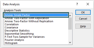
3: Click “OK” > the “ANOVA: Single Factor” window opens. Add the details as shown below.

Go to the “Input” group > enter the data range in the “Input Range” field as A1:C9, choose “Grouped By:” as “Columns”, and check/tick the “Labels in first row” [Note: The Alpha value will be 0.05 by default].
Now, go to the “Output Options” group > select the “Output Range:” option > enter the cell as F1 in the “Output Range:” field.

[Note:

To display the output in the current sheet, select the “Output Range:” option in the “Output Options” group and enter the target cell to show the ANOVA in Excel test result.
To display the output in a new spreadsheet, select the “New Worksheet Ply:” option in the “Output Options” group, and enter the target cell.]

4: Click “OK” in the “ANOVA: Single Factor” window. We will get the following output.

Output interpretation: We will now understand the ANOVA in Excel meaning of the above result.

The F value is 0.00121. It is less than the F crit value, 3.4668. And the p-value is 0.998, which is more than the Alpha value, 0.05. Thus, we cannot eliminate the null hypothesis that the mean values of the three datasets representing the three tests are not significantly different.

Two Way ANOVA Test In Excel

A two-way ANOVA test in Excel helps determine the effect of two independent variables on a dependent variable. We will use the following options from the “Data Analysis” window.

ANOVA: Two-Factor with Replication.
ANOVA: Two-Factor Without Replication.

#ANOVA: Two-Factor with Replication

The following table shows five men’s balanced diet intake, exercise frequency, and weight loss data.

The steps to find the Two-Way ANOVA Test using the ANOVA: Two-Factor with Replication are:

1: Select the “Data” tab > go to the “Analysis” group > click the “Data Analysis” option.

2: Once the Data Analysis window opens, choose the first option i.e., “ANOVA: Two-Factor With Replication”, from the “Analysis Tools” list.

3: Click “OK” > the “ANOVA: Two-Factor With Replication” window opens. Add the details as shown below.

Go to the “Input” group > enter the data range in the “Input Range” field as A2:D12 > enter 5 in the “Rows per sample:” field, as there are five men. [Note: The Alpha value will be 05 by default].
Now, go to the “Output Options” group > select the “Output Range:” option > enter the cell as G1 in the “Output Range:” field.

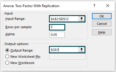
4: To get the output in the current sheet, set the “Output Range” as the target cell in the current sheet. Finally, click “OK” in the “ANOVA: Two-Factor With Replication” window. We will get the following output.

Output interpretation: We will now understand the ANOVA in Excel meaning of the above result.

Consider the last table, ANOVA. The Sample field refers to Exercise Frequency, and the Columns field indicates Balanced Diet Intake. Now observe the p-value.

The p-value of Exercise Frequency is 68E-05. It is statistically significant as it is less than the Alpha value of 0.05.
The p-value of Balanced Diet Intake is 01E-07. It is statistically significant as it is less than the Alpha value of 0.05.
The p-value for the interaction between Exercise Frequency and Balanced Diet Intake is 228173. So, it is not statistically significant as it is greater than the Alpha value of 0.05.

Thus, these observations indicate that both factors, Exercise Frequency and Balanced Diet Intake, have a statistically significant impact on weight loss. And they are the main effects in this example model.

Also, the significant p-values prove that the mean values for the five men sample data are not equal. The Average field in the SUMMARY table corroborates the above observation.

On the other hand, there is no interaction effect. So, whether a person exercises daily or weekly, it does not affect how they lose weight due to a balanced diet. Instead, the main effects are the section of the relationship between the independent and the dependent variables that do not get modified based on the other variables’ values.

#ANOVA: Two-Factor Without Replication

The two-factor ANOVA in Excel without replication is an extension of the single-factor ANOVA test, except there are two independent variables instead of one factor. Therefore, we can follow the above-explained steps to determine it. But the ANOVA test type in the Data Analysis window is “ANOVA: Two-Factor Without Replication”.

But, while the ANOVA test without replication helps analyze the effects of the independent variables on the dependent variable, we cannot review the interaction between them.

ANOVA In Excel Interpretation

The ANOVA in Excel results or output consists of two tables, SUMMARY and ANOVA.

The SUMMARY table shows the sample Count, Sum, Average, and Variance data for each group in the model.

Count: It is the number of samples in each group in the model.
Sum: It is the sum of values in each group in the model.
Average: The result obtained from dividing the Sum by Count for each group in the model.
Variance: The data points’ dispersion level from the respective group mean value.

The ANOVA table shows the values SS, df, MS, F, P-value, and F crit for each source of variation.

SS: It is the sum of squares for each source of variation.
df: It denotes the degree of freedom associated with each variance source.
MS: It shows the mean square.
F: It shows the F-statistic used during the null hypothesis test to determine the model’s significance. It is the result of dividing variation between the sample means and variation within the samples.
P-value: The probability determines the evidence against the null hypothesis.
F crit: The parameter stands for F critical. It is the F-statistic value at the threshold probability, Alpha, of wrongly eliminating a null hypothesis.

When we perform a test for ANOVA in Excel, we need to check the F and p-value in the result to interpret the output and determine the model’s significance.

We cannot eliminate the null hypothesis in a single-factor ANOVA test if the F value is less than the F crit value. Likewise, we cannot reject the null hypothesis if the p-value is higher than the Alpha value.

In a two-way ANOVA test with replication, the factor or independent variable with a significant p-value (i.e., a p-value less than the Alpha value) affects the dependent variable. And a significant p-value of Interaction indicates the relationship between an independent and the dependent variables gets modified based on the other independent variable value.

On the other hand, the ANOVA test interpretation remains the same for a two-way ANOVA test without replication, except there will be no interaction data to analyze.

Important Things To Note

ANOVA in Excel helps perform analysis of variance and tests such as null hypothesis testing for models involving three or more independent groups.
Enable the Analysis ToolPak add-in to get the Data Analysis feature added to the Data tab required to perform the ANOVA tests.
If the F value is less than the F crit value or the p-value is more than the Alpha value in a one-way ANOVA test, we cannot eliminate the null hypothesis.
The factor or independent variable with a significant p-value (i.e., a p-value less than the Alpha value) affects the dependent variable in a two-way ANOVA test.

Frequently Asked Questions

What is ANOVA in Excel used for?

ANOVA in Excel is used to check whether the mean values of various groups in a dataset are significantly different. It evaluates the effect of one or more independent variables or factors on a dependent variable by comparing the mean values of different samples.

Which ANOVA in Excel to use?

We can use the one-factor or two-factor ANOVA in Excel. And we have two options available for the two-factor or two-way ANOVA test, one with replication and the other without replication.

How to run an ANOVA in Excel?

We can run an ANOVA in Excel using the below steps:

Step 1: In the current worksheet, choose Data > Data Analysis to open the Data Analysis window.

Step 2: Select the ANOVA test we require to perform for our model from the Data Analysis window.

Once we choose the required ANOVA test from the three options highlighted in the above image and click OK, their respective dialog boxes pop up. Next, we will need to enter the input data and the location where we want to display the ANOVA test result i.e., whether in the current worksheet itself or a new worksheet and click OK to view the result.

What is F in ANOVA in Excel?

F in ANOVA in Excel is the parameter that determines the model significance in a null hypothesis.

Download Template

This article must help understand ANOVA in Excel, with its formula and examples. We can download the template here to use it instantly.

ANOVA In Excel Download

ANOVA In Excel