Add-ins In Excel

What Are Add-ins In Excel?

Add-ins in Excel allow users to extend the program’s functionality across various platforms that include Windows, Mac, etc. In addition, the users can add customized features and commands to the Excel application for easy access. Add-ins in Excel support better user interaction with Excel objects and enable them to manipulate their data in a spreadsheet more efficiently.

For example, the table below shows the amount of DEM (Deutschmark) in cell A2. We can convert it to Euros using the manage Add-ins in Excel and display the converted currency in cell D2.

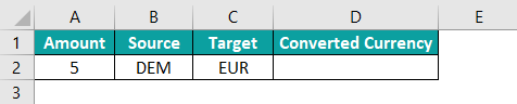
In this example, we can activate the Euro Currency Tools Add-ins to determine the required value.

[Note: In the image below, the Euro Currency Tools is already enabled. So, it is visible in the ribbon].

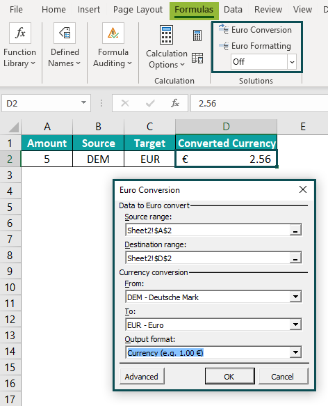
Select the “Formula” tab > go to the “Solutions” group > click the “Euro Conversion” option.

The “Euro Conversion” window pops up.

Enter the required details, as shown in the above image, and complete the required calculations. Then, click on “OK”. In cell D2, we have the converted amount.

Similarly, we can activate and show Add-ins in Excel ribbon, best suiting the requirements and daily task demands.

How To Install Add-ins In Excel?

When some of the Excel features are not visible in the Excel ribbon, we must first enable them.

The steps to install or enable Add-ins In Excel are:

Step 1: Select the “File” tab.

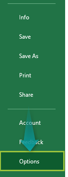
Step 2: In the File menu, choose “Options” from the file menu.

Step 3: The “Excel Options” window opens. On the left, click the “Add-ins” option, on the right, the “Manage” field should be “Excel Add-in” [If not, select from the drop-down], click on “Go…”, as shown below.

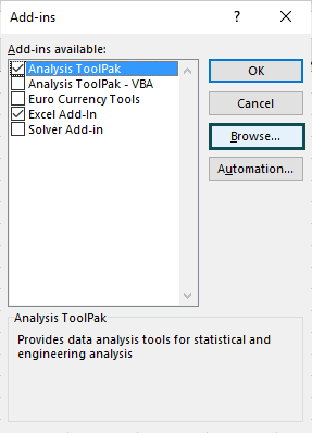
Step 4: The moment we press “Go…” the “Add-ins” window pops up. Check/tick the required Add-ins checkbox for the worksheet. For example, to access Data Analysis and Solver functionalities, choose “Analysis ToolPak” and “Solver Add-ins” from the list, as shown in the below image, and click “OK”.

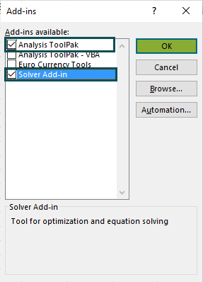
Now, the Data Analysis and Solver Add-ins are enabled and are visible in the Data tab.

Thus, we can install and manage Add-ins in Excel from the “File” tab and the “Add-ins” window.

Types Of Add-ins In Excel

There are three types of Add-ins in Excel, namely,

• Excel Add-ins.
• Downloadable Add-ins.
• Custom Add-ins.

#1 – Excel Add-in

These are the inbuilt Add-ins in Excel. They typically have the extensions, .xlam, .xla, and .xll.

Some examples are The Euro Currency Tools and Analysis ToolPak, seen in the previous sections.

#2 – Downloadable Add-ins

We can download some Add-ins from the internet to perform specific tasks.

For example, we can download from the Microsoft website and show Add-ins in Excel ribbon, using the steps explained in the previous section.

#3 – Custom Add-ins

We can use the Custom Add-ins to standardize our daily tasks. First, we use VBA code to build them.

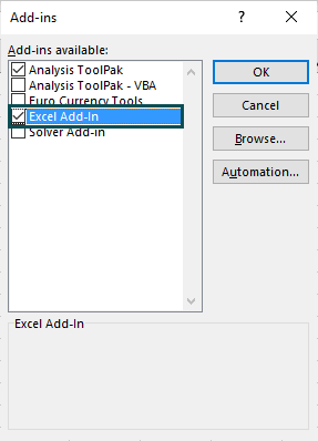
For example, the below image shows Custom Add-ins. It is visible in the Add-ins window because it is a VBA Macro saved as an Excel Add-in, as shown below.

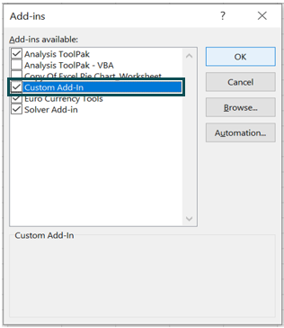
Therefore, whether it is an inbuilt, downloadable, or custom Add-ins, we must check/uncheck the respective Add-ins checkbox to enable/disable Add-ins in Excel.

The Data Analysis Add-in

The Data Analysis is one of the most-powerful Add-ins. It finds its application in finance, statistical data analysis, and engineering domains.

Once the Analysis ToolPak Add-ins are enabled, they will be in the Data tab.

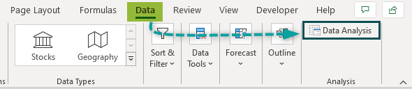
When we click the Data Analysis option, the Data Analysis window opens. Here, we can choose the required function and click OK to execute it.

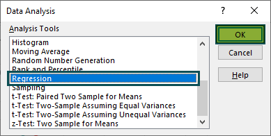
These Add-ins are useful when we need analysis, such as Regression and t-Tests.

Create Custom Functions And Install As An Excel Add-in

We will understand the Excel Add-in with some advanced scenarios. We will Create Custom Functions and Install as An Excel Add-in.

Example #1- Extract Comments From The Cells Of Excel

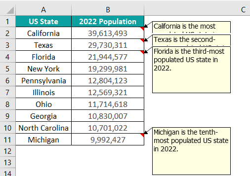
We will Extract Comments from The Cells Of Excel using the following data table.

The table with cells B2:B4 and B11 has comments, and we want to extract the comments from the specific cells into our worksheet.

The steps to Extract Comments by creating Excel Add-in are:

Step 1: Open a new workbook > select the “Developer” tab > go to the “Code” group > select the “Visual Basic” option, and the “Visual Basic Editor” window opens.  [Alternatively, use the shortcut keys, Alt+F11, to open the “Visual Basic Editor” window].

In the “Visual Basic Editor” window, select the “Insert” tab > click on the “Module” option, as shown below.

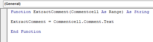
Step 2: The Module 1 window opens. Enter the custom function shown in the image below to build the Add-ins to extract the comments from the cells in our spreadsheet.

Function ExtractComment(Commentcell As Range) As String

ExtractComment = Commentcell.Comment.Text

End Function

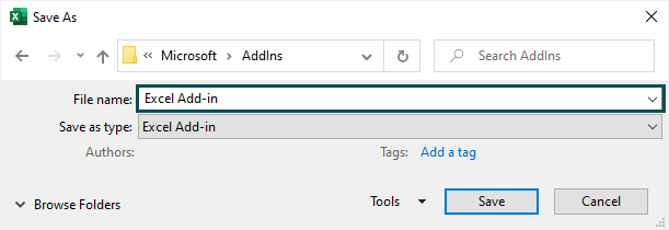
Step 3: Save the file as an Excel Add-in. [By default, the file gets saved in the Microsoft folder. But we can store it in any desired folder.

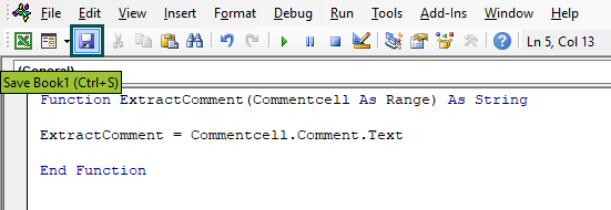
The “Save As” folder is shown below.

Step 4: Now, open our worksheet with cells containing the comments we want to extract, and using the Add-ins, open the Add-ins window.

Step 5: Click “Browse” in the Add-ins window to locate the folder where the saved workbook containing the VBA Macro is found.

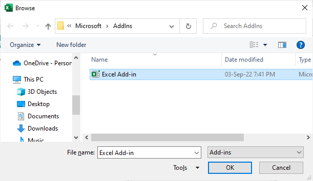
And once we click on “OK”, the workbook will appear in the list.

Click “OK” to close the Add-ins window.

Step 6: Now, in the worksheet with cells containing the comments, choose cell C2 and enter the custom function we created as =ExtractComment(B2). We will get the following output in cell C2.

[Note: Once we start typing the function name after the ‘=‘ sign, it will appear like the rest of the Excel functions beginning with the same letter as the custom function].

Step 7: Drag the formula from cell C2 to C11 using the fill handle to extract the comments from the remaining cells B3:B11.

In the above example, cells B2:B4 and B11 have comments, which the custom function extracts through the activated Excel Add-in. However, in cells C5:C10, the function returns #VALUE! Error because cells B5:B10 do not have comments.

Example #2- Hide/Unhide Worksheets In Excel

Add-ins in Excel allow us to hide/unhide worksheets, except the current spreadsheet. In such scenarios, we can create and add, Add-in icons to our Excel toolbar for later use.

The steps to Hide/Unhide Worksheets by creating Excel Add-in are:

Step 1: Open a new workbook à select the “Developer” tab > go to the “Code” group > select the “Visual Basic” option, and the “Visual Basic Editor” window opens.

In the “Visual Basic Editor” window, select the “Insert” tab > click on the “Module” option.

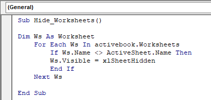
Step 2: The Module 1 window opens. Enter the VBA code shown in the image below to hide all worksheets, and save the workbook with the Excel Add-in file type.

Sub Hide_Worksheets()

Dim Ws As Worksheet
For Each Ws In activebook.Worksheets
If Ws.Name <> ActiveSheet.Name Then
Ws.Visible = xlSheetHidden
End If
Next Ws

End Sub

Step 3: Now, open the workbook where we want the Add-ins icon to hide worksheets. In the workbook, select the “File” tab > click the “Options” in the file menu.

Step 4: The “Excel Options” window opens. On the left, click the “Add-ins” option > on the right, click on “Go…”, as shown below.

Step 5: Click the “Browse” option in the Add-ins window.

Select the file with the VBA Macro to hide worksheets.

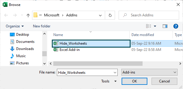
Once we click “OK”, the workbook gets listed, with its box checked in the Add-ins window.

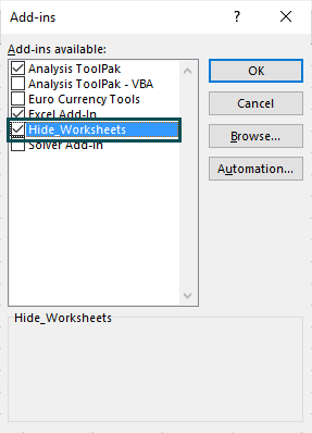
Click OK to close the Add-ins window.

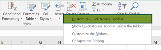
Step 6: Right-click on the Excel ribbon and choose the “Customize Quick Access Toolbar” option.

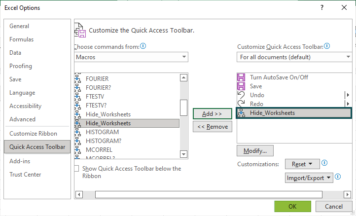
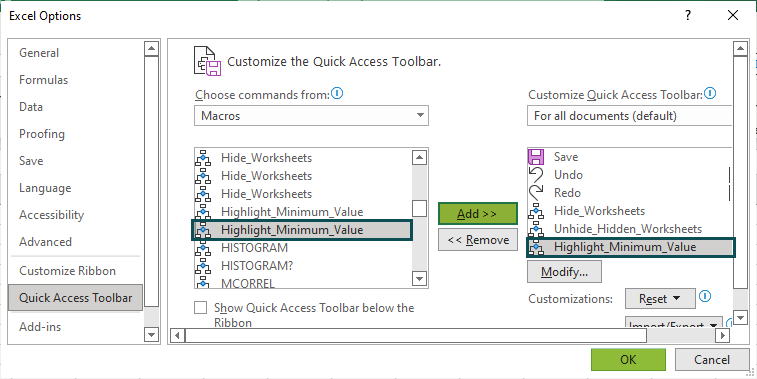
Step 7: The “Quick Access Toolbar” window pops up. Set the “Choose command from:” drop-down as “Macros” > select the “Hide_Worksheets” option > click on the “Add” button, as shown below.

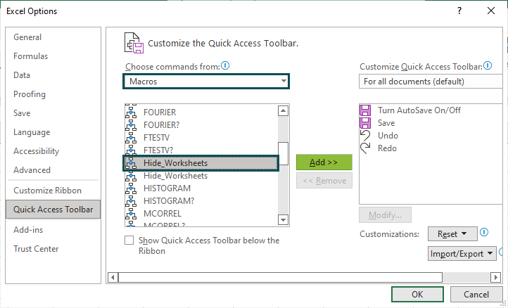
The chosen command gets added to the “Customize Quick Access Toolbar:” list.

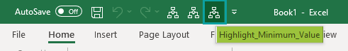
Once we click “OK”, we will get the Add-ins icon in the Excel ribbon, as shown below.

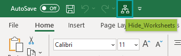
When we click the Hide_Worksheets Add-ins icon, all sheets are hidden except the active worksheet.

Step 8: Open another module and enter the VBA code, as shown below, to unhide worksheets and save the workbook with the file type Excel Add-in.

Sub Unhide_Hidden_Worksheets()

Dim Ws As Worksheet
For Each Ws In activebook.Worksheets
Ws.Visible = xlSheetVisible
Next Ws

End Sub

Step 9: Repeat steps 2 to 7 to get the Add-ins icon for Unhide Hidden Worksheets.

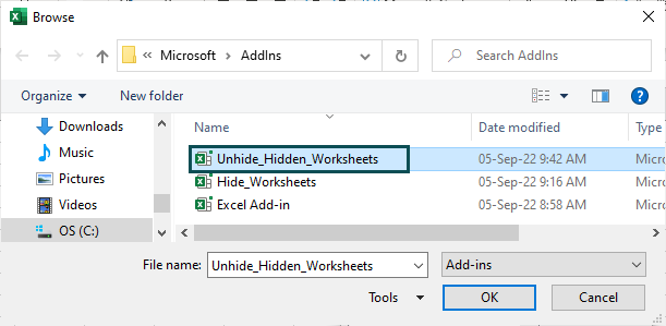
Open the workbook where we want to unhide worksheets. Then open the “Add-ins” window and click on “Browse”. Next, access the workbook containing the VBA code to unhide worksheets from the location where we saved the file.

Step 10: Once we click “OK”, the workbook gets listed, with its box checked in the Add-ins window.

Step 10: Now customize the “Quick Access Toolbar”.

Once we click “OK”, we will get the Add-ins icon in the Excel ribbon, as shown below.

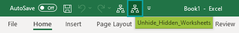
And, when we click on the Unhide_Hidden_WorkSheets Add-ins icon, all hidden worksheets will be unhidden or visible.

Example #3 – Add-ins In Excel To Perform Mathematical Calculations Over A Cell Range

We will use Add-ins in Excel to perform mathematical calculations over a cell range.

The following table shows the Physics marks of 10 students, and we have to find the least score. We must write a VBA Macro and create an Add-ins icon to determine the minimum value.

The steps to Perform Mathematical Calculations Over A Cell Range by creating Excel Add-in are:

Step 1: Open a new workbook and the “Visual Basic Editor”. Next, go to “Insert” > “Module”.

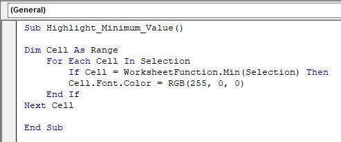
Enter the VBA code shown in the image below in the module window to show the least value in a cell range. Then, save the workbook as an Excel Add-in.

Sub Highlight_Minimum_Value()

Dim Cell As Range
For Each Cell In Selection
If Cell = WorksheetFunction.Min(Selection) Then
Cell.Font.Color = RGB(255, 0, 0)
End If
Next Cell

End Sub

Step 2: Open the workbook where we want to highlight the least score. Then open the Add-ins window and click on “Browse” to locate and add the saved Excel Add-in file to the Add-ins list.

Step 3: Now, right-click on the Excel ribbon and choose “Customize Quick Access Toolbar” to open the “Quick Access Toolbar”.

Once we click OK, we will get the Add-ins icon for Highlight_Minimum_Value in the Excel toolbar, as depicted below:

Step 4: Choose the cell range B2:B11 and click on the Add-ins icon for Highlight_Minimum_Value.

Once we click on the Add-ins icon, the least score gets highlighted in red, as shown below.

The output is shown above. Cell B7 has the minimum value score, highlighted in Red.

Important Things To Note

• Add-ins in Excel offer a few optional functions and features that are disabled by default in Excel. However, as per our requirement, we can enable them.
• We must always use the file extension as Excel Add-in while saving the Add-ins file.
• In the Add-ins window, we must choose the correct file while browsing to add an Add-ins.
• The best practice is to disable Add-ins in Excel by unchecking the corresponding boxes in the Add-ins window when not in use.

Frequently Asked Questions

Download Template

This article must help understand Add-ins with its formula and examples. You can download the template here to use it instantly.

Recommended Articles

This has been a guide to Add-ins in Excel. Here we add and enable/disable inbuilt add-in, download online, custom add-in (VBA), examples & downloadable excel template. You can learn more from the following articles – 

• Descriptive Statistics in Excel
• Regression Analysis In Excel
• Solver in Excel