SORTN in Google Sheets

What is SORTN in Google Sheets?

The SORTN function in Google Sheets returns a specified number of items from a data range that has been sorted based on one or more columns. It is very useful when you want to extract the top or bottom values from a dataset without sorting the entire table. It is so-called because it combines sorting and returns only a specific number (N) of the top or bottom rows, unlike SORT, which returns all rows.

For example, suppose we have a list of students and their scores, and wish to display only the top 3 scorers. We can use the SORTN function. It will pick those three entries with the highest scores and ignore the rest of the data. This helps in keeping your sheet clean and focused.

SORTN in Google Sheets returns a specific number of top or bottom rows from a dataset based on a defined sorting criterion.
Its syntax is as follows: =SORTN(range, [n], [display_ties_mode], [sort_column], [is_ascending], …)
The SORTN function doesn’t modify the original data, It creates a new sorted subset and supports sorting by multiple columns.
The function returns an #VALUE error if one uses an invalid column index or varied data types, it will return a #VALUE! error.
It’s especially useful for tasks like leaderboards or dashboards where only top results are needed.

Syntax

The syntax of the SORTN function is slightly more complex than other basic functions, but still easy to use.

=SORTN(range, [n], [display_ties_mode], [sort_column1, is_ascending1], …)

range – The range of data from which you want the sorted values.
n (optional) – The number of items you want the function to return. If omitted, it returns 1 item.
display_ties_mode (optional) – Determines how to handle ties:
- 0: Omit extra items in case of ties.
- 1: Include all tied items, which may result in more than n rows.
- 2: Remove duplicate rows
sort_column1, is_ascending1 (optional) – One or more pairs that define which columns to sort by and in which order:
- sort_column1 – The column number or range to sort on.
- is_ascending1 – TRUE to sort in ascending order, FALSE for descending.

How to Use SORTN Function in Google Sheets?

You can use the SORTN function in two ways:

Manually typing the SORTN formula.
Using the Google Sheets menu

Manually Entering the SORTN Function

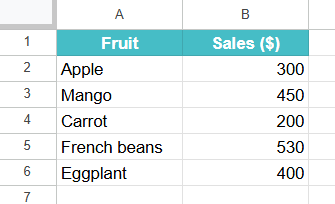
Let’s look at how to manually use the SORTN function to return the top 3 products with the highest sales from the sales information if a store.

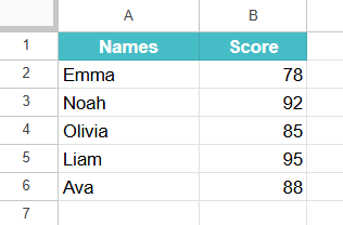
Step 1: We enter the product names in Column A and their sales numbers in Column B.

Step 2: To sort according to sales and get the top three products, in cell D1, type the following formula.

First, enter the = sign followed by the SORTN( function. Enter the required arguments in the order shown below. Close the braces and press Enter.

=SORTN(A2:B6, 3, 0, 2, FALSE)

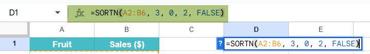
This returns the top 3 rows based on the second column (sales), sorted in descending order(FALSE).

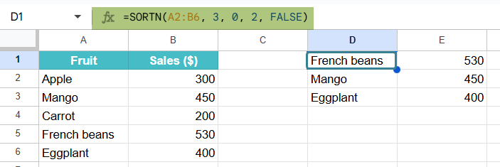
Step 3: Press Enter, and the top 3 products by sales will appear starting from cell D1.

Using the Google Sheets Menu Bar

To insert the SORTN function using the menu:

Click on the cell where you want the result to appear.
Go to Insert > Function > Lookup > SORTN.
Fill in the arguments using the helper prompts, just like in the formula bar.

Examples

To understand how the SORTN function works, let’s walk through some practical examples. The SORTN function is useful when you wish to extract only the top or bottom entries based on sorting logic.

Example #1

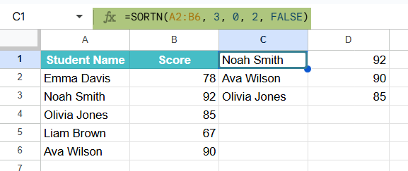
Consider a teacher who wishes to display only the top three students based on their scores using the SORTN function. Let us see how to do this.

Step 1: We enter the list of student names and their exam scores in Columns A and B of a spreadsheet.

SORTN function in Google Sheets Example 1

Step 2: Click on an empty cell and enter the following formula:

=SORTN(A2:B6, 3, 0, 2, FALSE)

SORTN function in Google Sheets Example 1-1

A2:B6 is the range that contains both student names and scores.
3 tells the function to return only the top 3 results.
0 specifies no special treatment for ties.
2 indicates that sorting should be based on the second column
FALSE sorts the results in descending order

Step 3: Press Enter. You’ll now see only the top 3 scoring students appear in the new cells.

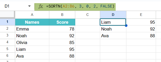
SORTN function in Google Sheets Example 1-2

The formula filters and displays just the highest scorers, making it easier to analyze results without manually sorting or hiding rows.

Example #2 – Sort the top 3 selling products each month, considering both sales quantity and revenue

Let us track the performance of various products from the monthly sales report of a store. There are two key metrics, which are the quantity sold, and revenue generated. We must display only the top 3 best-performing products, considering the revenue first, and then Quantity sold, if there is a tie. Let us use the SORTN function to extract and sort the data efficiently without altering the values.

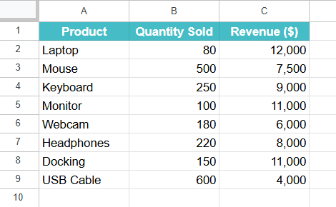
Step 1: Let us organize the data in three columns: Product Name, Quantity Sold, and Revenue. In this SORTN Google Sheets example, we will sort by SORTN Google Sheets multiple column.

SORTN function in Google Sheets Example 2

Step 2: Click on an empty cell to display the results. Begin typing the SORTN function. Enter the formula to sort and return the top 3 products:

=SORTN(A2:C10, 3, 0, 3, FALSE, 2, FALSE)

This is based on the syntax:

A2:C10 is the range

3 indicates that you want only the top 3 entries.
0 means no special handling for ties.
3, FALSE sorts by third column in descending order.
2, FALSE is a secondary sort through Quantity Sold in descending.

SORTN function in Google Sheets Example 2-1

Step 4: Press Enter. The top 3 products are displayed, sorted first by revenue, and then by quantity if revenues are tied.

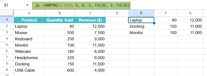
SORTN function in Google Sheets Example 2-2

This example highlights how the SORTN function can be used for multi-level sorting to generate top performers. Whether you’re analyzing sales by month, quarter, or region, this method saves time and gives valuable insights into your sales data.

Example #3 – Combining SORTN with Conditional Formatting to Highlight Top Performers

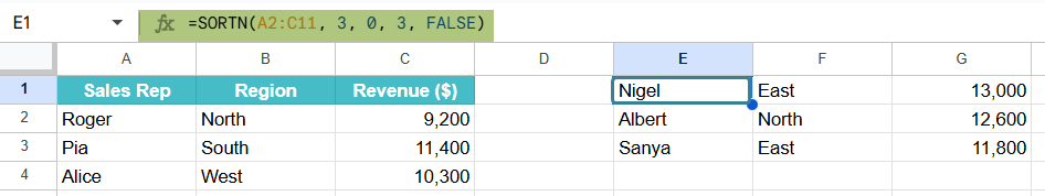
There is a sales team across different regions, and the company wishes to highlight the top performers based on total revenue visually. We list the top performers using SORTN and highlight their names to be automatically highlighted for quick visual reference.

This method makes it easy to present key performers in dashboards and team reviews without manually checking.

Step 1: Enter the sales data in Columns A to C.

SORTN function in Google Sheets Example 3

Step 2: In an empty cell, type the following formula for the top three representatives.

=SORTN(A2:C11, 3, 0, 3, FALSE)

A2:C11: range including names and revenue.
3: shows only the top 3 results.
3, FALSE: sorts by Revenue (third column) in descending order.

SORTN function in Google Sheets Example 3-1

Step 3: Press Enter for the result.

SORTN function in Google Sheets Example 3-2

Step 4: Let us add conditional formatting. This will add an automatic visual element, making it easy to read the sheet.First, select the range from A2:A11.

Go to Format > Conditional formatting.

SORTN function in Google Sheets Example 3-3

Step 5: under “Format cells if”, choose “Custom formula is“.

Enter this custom formula:

=COUNTIF($E$1:$E$3, A2)>0

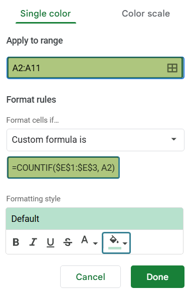
SORTN function in Google Sheets Example 3-4

This checks if the name in each row exists in the SORTN output. If yes, it applies the format. Press Done to see the result in the range. Instantly, your top 3 sales reps will be highlighted in the main list, automatically updating whenever revenue data changes.

SORTN function in Google Sheets Example 3-5

Important Things to Note

The SORTN function expects a rectangular range with rows and columns. If the range includes empty rows, the results might be inconsistent or incomplete.
If we reference a column number that doesn’t exist within the range, SORTN will return a #VALUE! Error.
The third argument in SORTN in Google Sheets controls how ties are treated. 0 will exclude ties after the specified number of rows, while 1 includes tied rows even if it exceeds the limit.
The function SORTN in Google Sheets only returns a sorted subset. The original data remains unchanged.

Frequently Asked Questions (FAQs)

Does the SORTN function work with text values?

The SORTN function can sort text values as long as they are within the specified range. When sorting by a column containing text, it uses alphabetical sorting. A->Z for ascending sort and Z-> A for descending sort. The column we’re sorting should contain consistent data types. If needed, we can combine it with ARRAYFORMULA or SORT for more better logic.

How is SORTN different from SORT in Google Sheets?

While both functions sort data, SORTN returns only a limited number of rows (N), hence the name. SORT shows the entire sorted list. SORTN is ideal when you only need the top or worst performers. It also supports tie-breaking and multiple sort criteria. However, SORT is more appropriate for displaying fully sorted tables.

What error messages can we get when using SORTN in Google Sheets?

SORTN may return a #VALUE! Error if:

We reference a column index outside the provided range.
The data contains inconsistent types (mix of text, numbers, etc.)
We try to sort a range that’s improperly structured or empty.

Download Template

This article must help understand SORTN Function in Google Sheets with its formulas and examples. You can download the template here to use it instantly.

SORTN Function in Google sheets Download

SORTN in Google Sheets