
What Is Conditional Formatting For Dates In Google Sheets?
Conditional formatting for dates in Google sheets is a method used to highlight or mark values based on conditions based on dates. It is easy to spot the value by using conditional formatting.
There are many conditional formatting rules with which we can format data, such as formula, cell type, text type and values etc., But, conditional formatting for dates, as the name suggests, conditions and filters the data with dates in Google sheets.
For example, consider the below table showing values in column A.

Now, we need to highlight years which are in the past in Google sheets.
To begin with, select the cell range and click on Format and then, select Conditional Formatting. Now, select Date is before in the Format cells if and then, click on In the past year to conditional format the data with dates.
Use this Conditional Formatting For Dates In Google Sheets Template to follow along with the examples in this article.
Download Excel TemplateNow, we will be able to see the result as shown in the below image.

Likewise, we can highlight the data with conditional formatting for dates in Google sheets.
In this article, let us learn how to use conditional formatting for dates in Google sheets with detailed examples.
How To Do Conditional Formatting For Dates In Google Sheets?
We can do conditional formatting for dates in Google sheets with the following steps.
The steps are:
Step 1: To begin with, we need to enter the cell range in the Google sheets. Next, we need to select the cell range which we want to format in Google sheets.
Step 2: Next, click on Format and then, select Conditional Formatting.
Step 3: The Conditional Formatting window appears on the right end of the screen.
Now, select the appropriate option in the Format cells if option and then, click on the necessary filter option to format the data with dates.
Now, we will be able to see the result.
Likewise, we can highlight the data with conditional formatting for dates in Google sheets.
Examples
Now, let us learn how to conditionally format the values for dates in Google sheets with detailed following examples.
Example #1 – Highlight Dates Due Today
For example, consider the below table showing name and expected delivery in columns A and B, respectively.

Now, we need to highlight dates due today in Google sheets.
The steps are:
Step 1: To begin with, we need to enter the cell range in the Google sheets. In this example, the data is available in the cell range A1:B6. Next, we need to select the cell range which we want to format in Google sheets. So, in this example, the data is available in the range A1:B6.
Step 2: Next, click on Format and then, select Conditional Formatting.
Step 3: The Conditional Formatting window appears on the right end of the screen.
Now, select Date is in the Format cells if option and then, click on today to format the data with dates.

Now, we will be able to see the result as shown in the below image.

Likewise, we can highlight the data with conditional formatting for dates in Google sheets.
Example #2 – Highlight Weekend Dates
For example, consider the below table showing days and dates in columns A and B, respectively.

Now, we need to highlight weekend dates in Google sheets.
The steps are:
Step 1: To begin with, we need to enter the cell range in the Google sheets. In this example, the data is available in the cell range A1:B5. Next, we need to select the cell range which we want to format in Google sheets. So, in this example, the data is available in the range A1:B5.
Step 2: Next, click on Format and then, select Conditional Formatting.
Step 3: The Conditional Formatting window appears on the right end of the screen.
Now, select Date is in the Format cells if option and then, click on in the past week to format the data with weekend dates.

Now, we will be able to see the result as shown in the below image.

Likewise, we can highlight the data with conditional formatting for dates in Google sheets.
Example #3 – Highlight Employee Absenteeism Dates In A Month
For example, consider the below table showing name and absent/leave in columns A, and B, respectively.

Now, we need to highlight employee absenteeism dates is a month in Google sheets. Assume that Henry is on leave on 20th August 2024.
The steps are:
Step 1: To begin with, we need to enter the cell range in the Google sheets. In this example, the data is available in the cell range A1:B6. Next, we need to select the cell range which we want to format in Google sheets. So, in this example, the data is available in the range A1:B6.
Step 2: Next, click on Format and then, select Conditional Formatting.
Step 3: The Conditional Formatting window appears on the right end of the screen.
Now, select Date is in the Format cells if option and then, click on exact date to format the data with dates.
Step 4: Now, enter 8/20/2024 in the Value or Formula box.
Now, we will be able to see the result as shown in the below image.

Likewise, we can highlight the data with conditional formatting for dates in Google sheets.
Example #4 – Highlight The US Festival Dtaes For 2024
For example, consider the below table showing days and dates in the month of July in columns A and B, respectively.

Now, we need to highlight the US festival dates for 2024 in the month of July in Google sheets. Assume that we want to highlight 4th of July.
The steps are:
Step 1: To begin with, we need to enter the cell range in the Google sheets. In this example, the data is available in the cell range A1:B6. Next, we need to select the cell range which we want to format in Google sheets. So, in this example, the data is available in the range A1:B6.
Step 2: Next, click on Format and then, select Conditional Formatting.
Step 3: The Conditional Formatting window appears on the right end of the screen.
Now, select ‘Date is’ in the Format cells if option and then, click on exact date to format the data with dates.
Step 4: Now, enter 4 in the Value or Formula option.
Now, we will be able to see the result as shown in the below image.

Likewise, we can highlight the US festival dates for 2024 in the month of July with conditional formatting for dates in Google sheets.
Important Things To Note
- Conditional formatting for dates in Google sheets, is a method to highlight the data with dates.
- We can highlight the data for dates in different inbuilt options. They are:
- Date is
- Date is before
- Date is after
Frequently Asked Questions (FAQs)
For example, consider the below table showing values in column A.
Now, we need to highlight years which are in the past in Google sheets.
The steps are:
Step 1: To begin with, we need to enter the cell range in the Google sheets. In this example, the data is available in the cell range A1:A3. Next, we need to select the cell range which we want to format in Google sheets. So, in this example, the data is available in the range A1:A3.
Step 2: Next, click on Format and then, select Conditional Formatting.
Step 3: The Conditional Formatting window appears on the right end of the screen.
Now, select Date is before in the Format cells if option and then, click on In the past year to format the data with dates.
Now, we will be able to see the result as shown in the below image.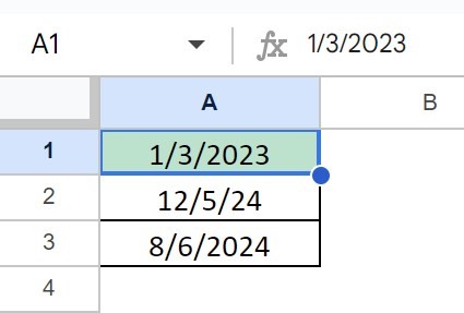
Conditional formatting in Google sheets for dates may not work properly if the data is not available in the cell range. Similarly, conditional formatting may not work if the exact date value mentioned in the conditional formatting window is not available in the data range.
We can clear conditional formatting in Google sheets in two ways.
Method 1:
1: We need to click anywhere on the cell range which is formatted conditionally.
2: Now, we will be able to see the Conditional Formatting window showing the formatting rule.
3: Simply click on the delete icon in the window to clear conditional formatting in Google sheets for dates.
Method 2:
Step 1: With the cell range in the sheet, click on Format and select Conditional formatting option.
Step 2: The Conditional formatting window opens up. Here, we can click on the delete icon to delete or clear conditional formatting in Google sheets for dates.
Use this Conditional Formatting For Dates In Google Sheets Template to follow along with the examples in this article.
Download Excel Template