
What Is DATE Function In Google Sheets?
The DATE Function in Google Sheets helps users to convert the year, month and day to a valid format Date, either by using obscure numeric values or cell references. The resulting date can be in the form of a serial number or an invalid format, then, we can change to the valid date format as required.
The Google Sheets DATE function helps us calculate the real-time dates by combining the DAY() and TODAY() functions. For example, we have the data below of a month, year and day. We will find the date using the values.
Use this DATE Function In Google Sheets Template to follow along with the examples in this article.
Download Excel Template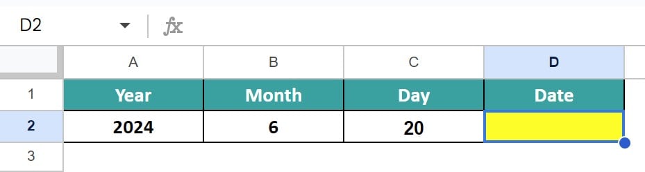
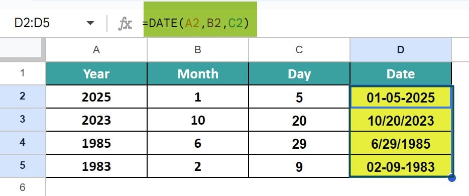
Select cell D2, enter the formula =date(A2,B2,C2) and press “Enter”, as shown below.

We get the output shown above in the already existing date format. We see the order of the arguments entered are in sequence, however, the resulting date appeared in the valid date format as mm/dd/yy.
Key Takeaways
- The DATE function in Google Sheets takes the day, month and year as input and returns the Date in a valid format or any other acceptable date format, which can be changed to a valid format.
- The connected functions to the DATE function are DATEVALUE(), MONTH(), DATEDIF(), EOMONTH(), EDATE functions, etc.
- We can use the Day() and the Today() functions to get the real-time dates, which means that once we enter these functions with the Date function, whenever we open the worksheet we will get the refreshed current date.
- We can create a list of sequential dates and also calculate the number of days between two dates by subtracting them.
Date() Google Sheets Formula
The syntax of the Date Google Sheets Formula is,

The three mandatory arguments of the Date Google Sheets Formula are,
- year: The year argument includes the cell value or the reference.
- month: It can be a positive or negative number representing the month from 1 to 12.
- day: The day’s value can be positive or negative and denotes the day from 1 to 28, 29, 30 or 31, again, depending on the month, whether its an even or an odd month, normal or a leap year, for February’s dates.
How To Use Date Function In Google Sheets?
We can use the DATE function In Google Sheets in 2 ways, namely,
- Access from the Google Sheets ribbon.
- Enter in the worksheet manually.
Method #1 – Access from the Google Sheets –
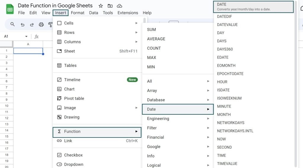
Step 1: Choose an empty cell for the output – select the “Insert” tab – click the “Function” option right arrow – click the “Date” option right arrow – select the “DATE” function, as shown below.
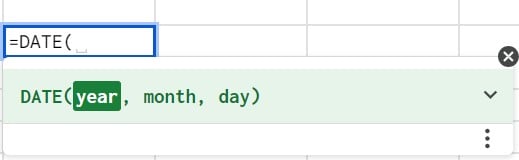
Step 2: The “DATE” formula appears, as shown below. Enter the argument as the cell reference.
Method #2 – Enter in the worksheet manually –
Step 1: Select an empty cell for the output.
Step 2: Type =DATE( in the cell. [Alternatively, type =D or =DA and double-click the DATE function from the Google Sheets suggestions.]
Step 3: Enter the arguments as cell values or cell references and close the brackets.
Step 4: Press Enter to view the outcome.
Examples
Let us learn to use the Date function in Google Sheets with some examples.
Example #1 – Using the DATE Function with Cell References in Google Sheets
The below table shows the random year, month, and day in columns A, B, C, and D, respectively. We need to find the date using the DATE function but with cell references of the values.

The steps to use the DATE Function with Cell References in Google Sheets of the values are,
Step 1: Select cell D1 and enter the formula =date(A2,B2,C2), where the argument values are cell references of cells A2, B2 and C2, as shown below.

Step 2: Press “Enter” to get the first output.
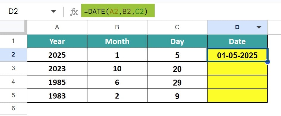
Step 3: Drag the formula from cell D2 to D5 using the fill handle.
Example #2 – Using the DATE Function to Display Real-Time Values in Google Sheets
The below table consists of a year and month. We will find the date using the DATE(), Day() and the Today() functions, which will always display the current date or the real-time date values whenever we open the Google Sheets.

The procedure to use the DATE Function to Display Real-Time Values in Google Sheets is,
Select cell C2 and enter the formula =Date(A2,B2,Day(Today()))
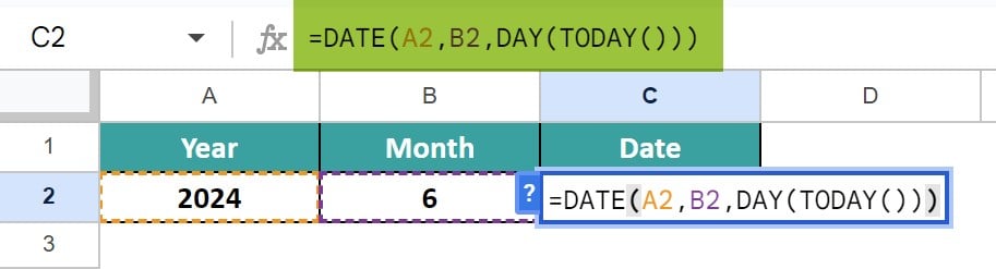
Press “Enter” to get the output, as shown below.
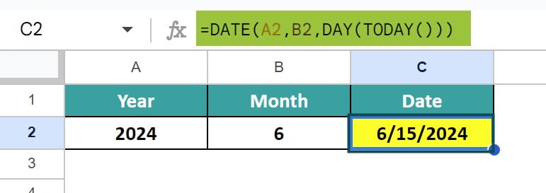
Output Observation: The formula shows how to find the real-time date.
- First, the Today() function doesn’t need any values, it displays the current date.
- Next, the Day() function needs the Date argument as a value or cell reference to only retrieve the day from the date. Here, we are not providing any date, but the Today() function’s result. Hence, the Day() function will always display the current day derived from the date of the Today() functions result.
Example #3 – Using Obscure Numerical Values with DATE in Google Sheets
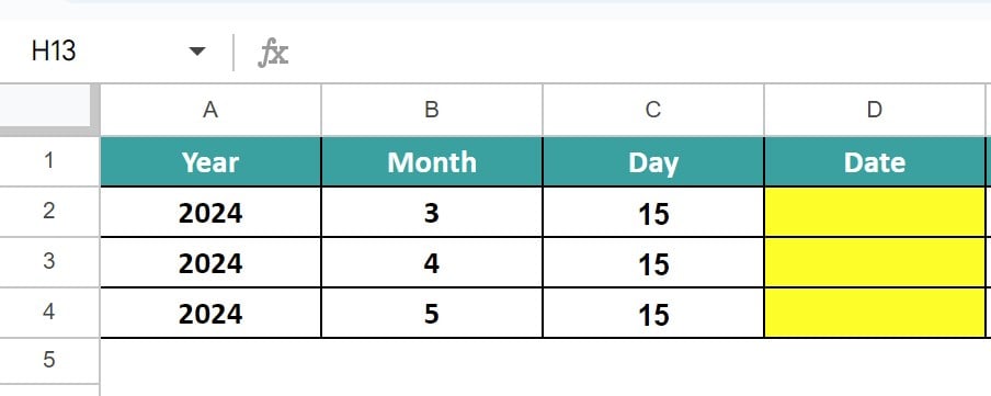
The below table consists of a year, month and day. We will find the date using the DATE() function, by using the values from the dataset and not any cell references or formula results. We have taken the same dates of 3 consecutive months.
The steps to use Obscure Numerical Values with DATE in Google Sheets are,
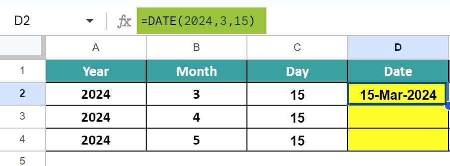
Step 1: Select cell C2, enter the formula =Date(2024,3,15) and press “Enter”. We get the output shown below.
[Note: For better understanding, we have used the long date format for date results.]
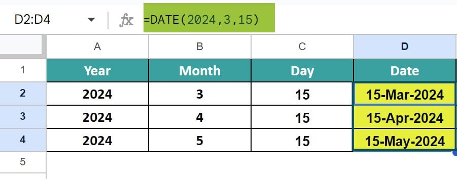
Step 2: Drag the formula from cell D2 to D4 using the fill handle. We get the same results, which are incorrect as per the dataset, as we have entered numeric values and not cell references.
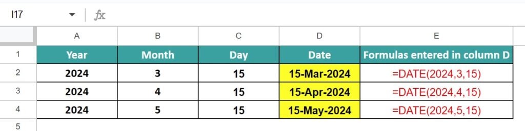
Step 3: Therefore, in such scenarios, we must enter the formula manually. Select cell D3 and D4 and enter the formulas =DATE(2024,4,15) and =DATE(2024,5,15), respectively, to get the output shown in the below image.
[Note: Column E is for our reference, with the formulas used in the corresponding cells in column D.]
Example #4 – Using DATE Function for a leap year
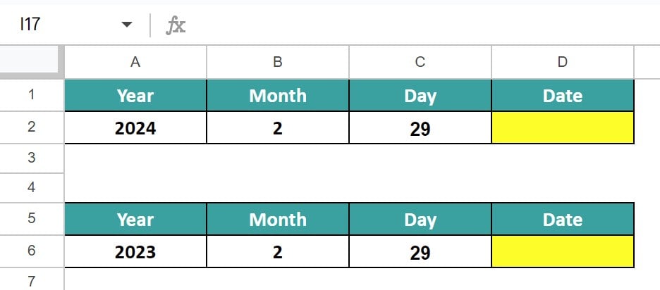
Consider the two data tables given below. Both tables have same days of the month of February, but the years are different. One of the years, is a leap year. We will find the date using the Date function and see what happens for the year that is not a leap year.
The steps to find the date using Google Sheets DATE function are,
Step 1: Select cell D2, enter the formula =date(A2,B2,C2) and press “Enter”.
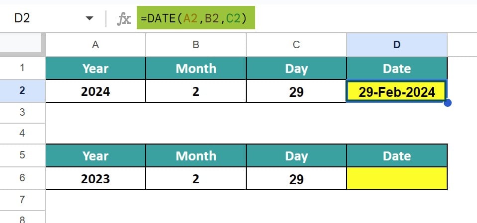
Step 2: Select cell D6, enter the formula =date(A6,B6,C6) and press “Enter”.
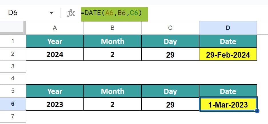
Output Observation:
- In cell D2, the output is normal as the year 2024 is a leap year. However, since the year 2023 is not a leap year and the month has only 28 days, the date formula counted 28+1 and returned the next date, i.e., March 1st, as the output in cell D6.
- If we enter 31 days for even months, then, the formula will add 30+1, i.e., the DATE would roll the date forward into the next month.
Important Things To Note
- If the DATE function returns a date serial number, then, we must format the result as a date to display the date format.
- #N/A occurs when any one of the arguments are not provided.
- The date argument range must be greater than or equal to 0, or else we get the #NUM! error.
- #VALUE! error occurs when the argument passed is non-numeric.
Frequently Asked Questions (FAQs)
We often forget in which category a function falls, here, the “DATE” function. Then, we can insert the function as follows:
Choose an empty cell – select the “Insert” tab – click the “Function” option right arrow – click the “All” option right arrow – select the “DATE” function, as shown below.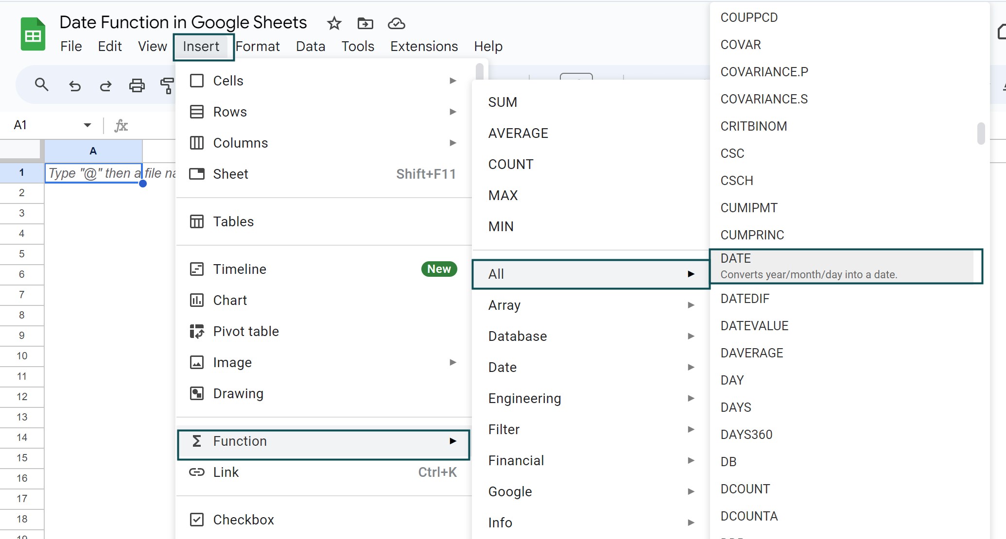
However, as always, entering the function manually is the best way to avoid confusion.
Alternatively, we can find the Functions icon to insert the DATE function in Google Sheets by following the path shown below.
Choose an empty cell – click the “More” option represented by the three vertical dots at the end of the toolbar, as shown below.
A list of icons appears when we click the “More” option. Here, click the “Functions” icon, as shown below.
Here, click the “Functions” option – click the “All” option right arrow à select the “DATE” function, as shown below.
A few reasons the Date function in Google Sheets may not work are,
a. One of the arguments are not provided or is less than 0.
b. If the date entered is not in valid format, then, we will get an error.
c. When we use the numeric values as cell arguments, ensure to enter the formulas in each result cell manually. The Drag and drop will not work and return incorrect dates.
Download Tempalte
Use this DATE Function In Google Sheets Template to follow along with the examples in this article.
Download Excel Template