
What Is XLOOKUP With Multiple Criteria In Google Sheets?
XLOOKUP with Multiple Criteria in Google Sheets looks for a specific value in a dataset and returns the value from another column with an exact, partial, or approximate match fulfilling multiple conditions or criteria.
The Google Sheets XLOOKUP with Multiple Criteria allows users to search for the desired value from the horizontal and vertical datasets, i.e., both to the left and right of the search values in rows and columns. We can perform XLOOKUP using Boolean Expressions, Concatenation, etc.
Use this XLOOKUP With Multiple Criteria In Google Sheets Template to follow along with the examples in this article.
Download Excel TemplateFor instance, we have the data of Planets, their position from the Sun and the number of moons they have. We have also created another table with out criteria for easy access in cells E2:F4. We will find the Moon count using the multiple conditions, i.e., its position from sun and the planets name, here, Earth.

Select cell F7, enter the formula =XLOOKUP(1,(A2:A9=F3)*(B2:B9=F4),C2:C9) and execute it as an array formula, i.e., press “Ctrl+Shift+Enter”.
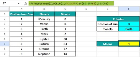
The output is shown above as 1, as the Earth has one moon.
Key Takeaways
- XLOOKUP with multiple criteria in Google Sheets searches a range of cells or a table array for a given value and returns an exact, partial, or approximate match from another column horizontally and vertically.
- In Google Sheets, XLOOKUP is a more advanced form of VLOOKUP and HLOOKUP. It outperforms VLOOKUP in terms of flexibility and variety.
- XLOOKUP can retrieve the values from left to the right, right to left, top to bottom, and bottom to top. Hence, the order of the data is not a matter of concern.
- Instead of providing row index number or column index number, we can provide the cell range.
XLOOKUP() Google Sheets Formula
The syntax of XLOOKUP Google Sheets formula is,
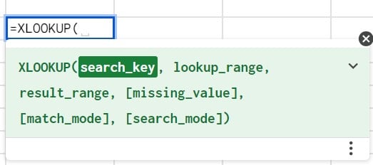
The syntax for XLOOKUP looks similar to VLOOKUP with additional parameters. XLOOKUP has six parameters where three are mandatory and the remaining three are optional.
The arguments of XLOOKUP Google Sheets formula are,
- search_key: The value for which we are trying to retrieve the result from return_range. It is a mandatory argument.
- lookup_range: It is either range of cells or a table array where we search for the search_key. It is also a mandatory argument.
- return_range: It is the array from which we need to get the desired result for the search_key. It is also a mandatory argument.
- [missing value]: If the search_key is not in the lookup_range, it results in a #N/A error. However, we can provide and get an alternative result here instead of the default #N/A error. This is an optional argument.
- [match_mode]: In this argument, we must specify the kind of match we need to do:
- 0 – It will search for the exact match of the search_key in the lookup_range. If nothing is specified, 0 will be the default input.-1 – It will search for an exact match. But if not found, it will look for the next smaller item than the search_key.1 – It will search for an exact match. But if not found, it will look for the next larger item than the search_key.
- 2 – It will perform a partial match using wildcard characters, like an asterisk (*) and tilt (~).
- [search_mode]: Here, we specify how the XLOOKUP searches for the search_key:
- 1 – It is the default searching option. It will allow the XLOOKUP to start searching from top to bottom in the lookup_range.-1 – It will search from bottom to top. It is helpful to find the last matching result for the search_key.2 – It will perform the binary searching for the data sorted in ascending order. If not sorted, we will get either the wrong result or an error.
- -2 – It will perform the binary searching for the data sorted in descending order. If not sorted, we will get either the wrong result or an error.
How To Use XLOOKUP With Multiple Criteria In Google Sheets?
We can use the XLOOKUP with Multiple Criteria in Google Sheets using following ways, namely,
- Boolean Expressions – Here, it simply finds if the output is True or False.
The syntax will be,
=XLOOKUP(1, (lookup_range1 = search_key1) * (lookup_range2 = search_key2) * (…), return_range)
- Concatenation – Here, we combine all the criterias in as single search_key using the Concatenate operator “&”.
The syntax will be,
= XLOOKUP(search_key1 & search_key2 & …, lookup_range1 & lookup_range2 & …, return_range)
Examples
We will consider some XLOOKUP with Multiple Criteria in Google Sheets examples.
Example #1 – Multiple Criteria Using Concatenation
We have the employee details such as, ID, Name, department and the wages they earned across months in the dataset given below. Also, another table with criterias and result cells.
We will find XLOOKUP with multiple criteria using the Concatenation method, i.e., using the Concatenate symbol “&” to get the employee’s name using the emp ID and the department.

The steps to find the emp name using XLOOKUP multiple criteria are,
Step 1: Select cell E13 and enter the formula =XLOOKUP(B14&B15,A2:A11&B2:B11,C2:C11, as shown below.
[Note: We have inserted the multiple criteria cells, B14 and B15, and their respective cell ranges, A2:A11 and B2:B11, using concatenate symbol “&”.]

Step 2: Press “Ctrl+Shift+Enter” to execute as an array formula. Now, the formula changes to =ArrayFormula(XLOOKUP(B14&B15,A2:A11&B2:B11,C2:C11)), as shown below.

Step 3: Press “Enter” to get the employee’s name, as shown below.

Example #2 – Multiple Criteria Using Boolean Expressions.
Consider the data of Example 1 of the employee details in the dataset given below. Also, another table with criterias and result cells.
We will find XLOOKUP with multiple criteria using the Boolean Expressions method, to find the April Sales and the department using the emp name and the emp ID.

The steps to find the April sales and dept name using XLOOKUP multiple criteria are,
Step 1: Select cell L5, enter the formula =XLOOKUP(1,(B2:B11=L3)*(C2:C11=L2),G2:G11), press “Ctrl+Shift+Enter” to execute as an array and press “Enter”, as shown below.
[Note: We can insert the multiple criteria cells in any order, here cells L2 and L3, and their respective cell ranges, B2:B11 and C2:C11, using Boolean expression “*”.]

Step 2: Select cell L6, enter the formula =XLOOKUP(1,(B2:B11=L3)*(C2:C11=L2),A2:A11), press “Ctrl+Shift+Enter” to execute as an array and press “Enter”, as shown below.
[Note: Here, XLOOKUP searches for columns towards the left of the search_key too.]
We see we can retrieve the required data using the XLOOKUP multiple criteria.

Example #3 – Approximate Match
We have the data below of employees for 2 months and their bonus received according to their respective sales for the months. There is another table with the criterias and the result cells. Let us apply the XLOOKUP multiple criterias to find the bonus percentage according to a different sales value.

The procedure to find the approximate match using the XLOOKUP is,
Select cell G6, enter the formula =XLOOKUP(G4,if(B2:B11=G3,C2:C11),D2:D11,,-1), press “Ctrl+Shift+Enter” to execute as an array and press “Enter”, as shown below.

We can see the bonus % as 10% even though the sales value is 14,000. Now, in the dataset the employee Mirel has two values 12,000 for 10% and 27,000 for 20% and the formula searches for an approximate match between these two values. However, the next value for 15,000 is 12% which is more than the sales value 14,000. Therefore, it returns the output as 10%.
Example #4 – Partial Match
The data below consists of a list of fruits and their amount in a specific month. We will find the partial match using the XLOOKUP function. We also have another table with criteria and result cells.

The procedure to find the partial match using the XLOOKUP is,
Select cell G6, enter the formula =XLOOKUP(1,search(H2,A2:A8)*(B2:B8=H3),C2:C8,,2), press “Ctrl+Shift+Enter” to execute as an array and press “Enter”, as shown below.

We see the output as $350. The match_mode value 2 will perform a partial match.
Important Things To Note
- By default, XLOOKUP looks for the exact match and does not require mentioning the match_mode argument as 0.
- It allows you to specify a range of cells as the return_range instead of just a column index.
- If we do not find the search_key, then we get an #N/A error.
Frequently Asked Questions (FAQs)
The difference between the HLOOKUP, VLOOKUP and XLOOKUP are,
a) HLOOKUP
• H stands for “Horizontal” and the function performs a horizontal lookup.
• It searches the rows of a table and returns a specified value from a row. Therefore, we must supply the row index number as its third argument.
b) VLOOKUP
• V stands for “Vertical” and the function performs a vertical lookup.
• It searches the columns of a table and returns a specified value from a column. Therefore, we must supply the column index number as its third argument.
c) XLOOKUP
• It can retrieve the value from both horizontal and vertical datasets as it looks up both rows and columns and returns a specified value. XLOOKUP can look up data from an array on the left side of the search_key.
• The function can return value from a range of cells, not just a column or row.
A few reasons the XLOOKUP with multiple criteria in Google Sheets may not work are,
• The selected cell range is incorrect.
• We have not executed the formula as array. We must press “Ctrl+Shift+Enter”.
• We have not provided the match_mode correctly.
The XLOOKUP function in Google Sheets is inserted as shown below,
Choose a cell – select the “Insert” tab – click the “Function” option right arrow – click the “Lookup” right arrow – select the “XLOOKUP” function, as shown below.
Use this XLOOKUP With Multiple Criteria In Google Sheets Template to follow along with the examples in this article.
Download Excel TemplateRecommended Articles
Continue with these related resources when you want the next practical step in this topic.
- LOOKUP in Google Sheets
- HLOOKUP In Google Sheets
- VLOOKUP Table Array In Google Sheets
- VLOOKUP True In Google Sheets
- INDEX MATCH Function In Google Sheets
Explore the full Google Sheets Lookup Functions guide or browse Google Sheets Resources.