
What Is Count Colored Cells In Google Sheets?
The Count Colored Cells in Google Sheets helps users count the colored cells and calculate the total number of cells in a chosen range. We can also filter and count the cells highlighted in a specific color in the given range. In the Count Google Sheets Colored Cells, users can apply the feature to count cells by color while analyzing sales reports and financial statements containing categories of data with different color codes.
For example, the table below lists students and their teams where each team appears highlighted in a unique color. We have applied the filter feature for the headers, “Student” and “Team”. Let us count the column B cells highlighted in each color and display the outcome in cell B13.
Use this Count Colored Cells In Google Sheets Template to follow along with the examples in this article.
Download Excel Template
Select cell B13, enter the formula =subtotal(2,B2:B11), press “Enter”. We get the output as 10 because there is a total of 10 values.

Now, follow the path shown in the image below, i.e., “filter by color à orange”. So, once we click on the required color, the corresponding cells in the chosen cell range get filtered and displayed. And we can view the total number of visible cells in the selected color in the target cell.

Then we get the output shown below. The count of the orange-colored cells is 4.

Key Takeaways
- The Count Colored Cells In Google Sheets methods help one to calculate the total number of colored cells in a given range based on the specified shade.
- Users can utilize the techniques to count colored cells in a range while working with financial figures in spreadsheets containing data categorized using colors which is helpful while generating reports according to the required colors.
- We can apply the Filter option with the SUBTOTAL function, conditional formatting with COUNTIF or the Power Tools from the Add-ons, to count the total number of colored cells in a given column range.
- We can count blank and non-empty cells by background and font colors in a given cell range.
Top 3 Methods To Count Cells In Google Sheets
We can Count Colored Cells in Google Sheets using the top 3 methods, namely,
- Count Colored Cells using Conditional Formatting and COUNTIF.
- Count Colored Cells Using SUBTOTAL Function.
- Count Colored Cells Using Add-on.
Let us consider each method with a specific example in the following sections.
Method #1 – Count Colored Cells using Conditional Formatting and COUNTIF
For example, the table below lists different smartphones and the quantity sold. We will Count Colored Cells using Conditional Formatting and COUNTIF.

The steps to Count Colored Cells using Conditional Formatting and COUNTIF are as follows:
Step 1: First, let us apply “Conditional formatting”, as follows:
Choose the data range A2:B7, select the “Format” tab – click the “Conditional formatting” option. When the “Conditional format rule” pane opens on the right, click the “Add another rule” option, as shown below.

Step 2: Now, select the “Single color” tab and under the “Format rules” section,
- First, click the “format if…” drop-down, select the “greater than or equal to” option and enter 30 in the “Value” field that appears as soon as we select one of the options from the drop-down.
- Next, in the “Formatting style” options, select the color “Cyan” from the “Fill color” option.
- Finally, click the “Done” button, as shown below.

We get the output, shown in the above image.
Step 3: Now let us use the COUNTIF formula to count the number of formatted colored cells.
Select cell E4, enter the formula =COUNTIF(B2:B7,”>=30″) and press “Enter”.

We can see the output of the count of the colored cells w.r.t, the conditional formatting and the COUNTIF(), as shown below.

Method #2 – Count Colored Cells Using SUBTOTAL Function
We will Count Colored Cells Using SUBTOTAL Function and the Filter option.
The dataset given below consists of fruits, their grades and order dates. The rows of data are highlighted in different colors based on the order dates.
Consider the requirement to count the number of cells in column C based on each color and display the output in cell B14.

The steps to Count Colored Cells Using SUBTOTAL Function and the Filter method are as follows:
1: Choose cells A1:C1 – select the “Data” tab – click the “Create a filter” option, as shown below.

In the selected cell range, the filters appear right next to the headers, as shown below.

2: Choose cell B14 and enter the formula =SUBTOTAL( and select the function_code as per the requirement, here 2, as we need to count the cells.

3: Now, complete the formula as =SUBTOTAL(2,C2:C11).

4: Press Enter. The SUBTOTAL() counts the total number of visible cells in the cell range C2:C11 and returns the output, 10.

5: Click the column C filter – select the “Filter by Color” option right-arrow – click the “Fill- Color” option right arrow – select the “Yellow” color, as shown below.

Once we click the required color, the corresponding cells get filtered in the chosen range. So, the SUBTOTAL() in cell B14 will return the updated count of the filtered cells, as shown below.

Likewise, we can utilize the Filter option to filter by the required color, one at a time, to count the corresponding number of visible cells in the chosen cell range. For example, if we select the “Orange” color, then, we get the following output.

Method #3 – Count Colored Cells Using Add-on
We will now Count Colored Cells Using Add-on using the Method 2 example; hence, this time use the entire dataset.

The steps to Count Colored Cells Using Add-on are as follows:
Step 1: First ensure we have the needed Add-ons. Therefore, select the “Extensions” tab – click the “Add-ons” right-arrow – select the “Get add-ons” option, as shown below.

Step 2: The “Google Workspace Marketplace” window appears. There, type “Power Tools” in the search bar, select the software and install it.

Once the “Power Tools” software is installed, we will get the new option in the “Extensions” tab, as shown below.

Step 3: Let us now count the required colored cells in the dataset.
Select cells A1:C11 à select the “Extensions” tab – click the “Power Tools” right-arrow – select the “Start” option, as shown below.

Step 4: The “Power Tools” pane appears on the right.
- Click the “Calculate cells based on their colors” option drop-down.

- Select the “Function by color” option.

Step 5: Choose the options as follows:
- Select the “One Color” menu.
- Choose A1:C11 in the “Select range:” field.
- Choose the “Orange” color in the “Select Color:” field, rest of the options, leave it as it is.
- From the “Use function:” drop-down, choose the “COUNTA (text)” function.
- Next, select cell A13 for the output in the “Paste results to:” field.
- Finally, click the “Insert function” button at the bottom of the “Power Tools” window.

We will get the count of the orange-colored cells in the output cell A13 as 9, as shown below.

Step 6: Let us test the method for another scenario. Choose the options as follows:
- Select the “One Color” menu.
- Choose A1:C11 in the “Select range:” field.
- Choose the “Yellow” color in the “Select Color:” field, rest of the options, leave it as it is.
- From the “Use function:” drop-down, choose the “COUNTA (text)” function.
- Select cell C13 for the output in the “Paste results to:” field.
- Finally, click the “Insert function” button at the bottom of the “Power Tools” window.

We get the output as shown above.
Important Things To Note
- We can count cells by color in Google Sheets using the SUBTOTAL() when the source cell range lies in one column, and the cells in the specified cell range contain numeric values.
- Ensure to install Add-ons, else we will be unable to perform the count on colored cells using the Add-ons method.
Frequently Asked Questions (FAQs)
We insert the COUNTIF function in Google Sheets as follows:
Choose an empty cell for the output – select the “Insert” tab – click the “Function” option right arrow – click the “Math” option right arrow- select the “COUNTIF” function, as shown below.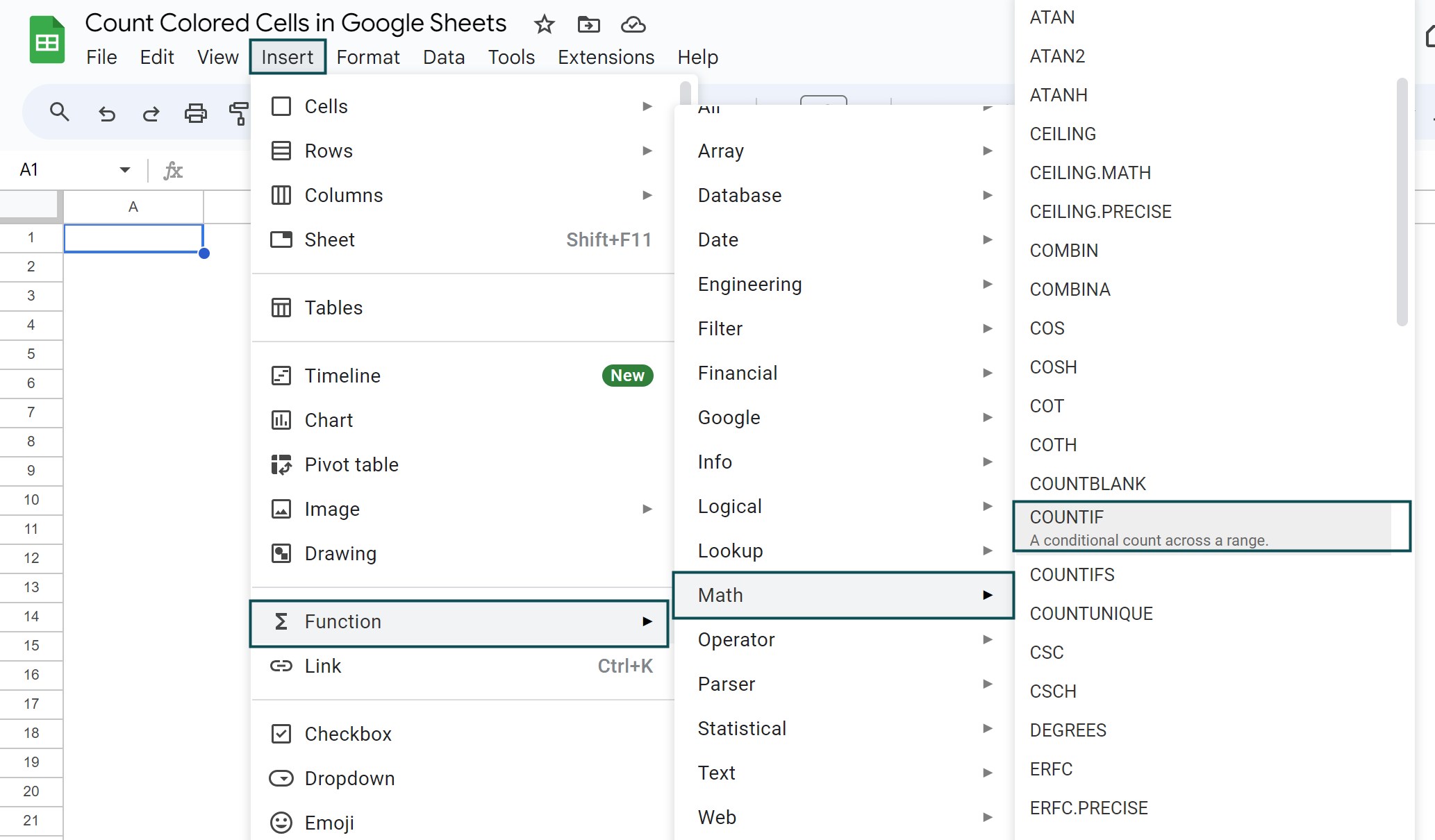
We can insert the COUNT functions such as, COUNTIF, COUNTIFS, COUNTBLANK, COUNTUNIQUE, etc. using the path shown above.
We insert the SUBTOTAL function in Google Sheets as follows:
Choose an empty cell for the output à select the “Insert” tab – click the “Function” option right arrow -click the “Math” option right arrow -select the “SUBTOTAL” function, as shown below.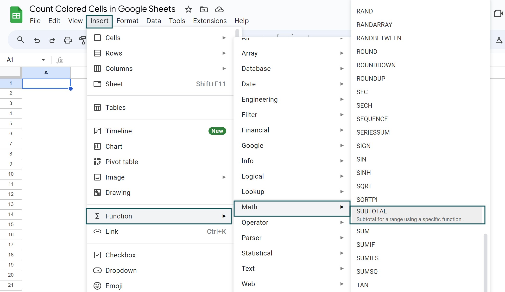
A few reasons the Count Colored Cells in Google Sheets may not work are as follows:
a. The formatting applied on the dataset is modified or deleted.
b. The dataset where the conditional formatting is applied is modified or deleted.
c. The right function_code is not selected in the “SUBTOTAL” function.
d. The Add-ons are not installed to perform the count of colored cells.
e. The data filters applied are removed. So, we are unable to filter by color.
Use this Count Colored Cells In Google Sheets Template to follow along with the examples in this article.
Download Excel Template