
What is ISOWEEKNUM in Google Sheets?
The ISOWEEKNUM function in Google Sheets returns the ISO week number for a given date(1-53). Unlike the regular WEEKNUM function, which allows weeks to start on Sunday or Monday, the ISOWEEKNUM function follows the international ISO standard, where each week begins on Monday and week 1 is defined as the week that includes January 4th or the first Thursday of the year.
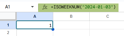
This function is very useful when you’re working across time zones and borders. It can be used when you have international teams, business reports, or requirements where time-based tracking that aligns with ISO calendars is necessary. It ensures consistency by sticking to a universally accepted week format. For example, using =ISOWEEKNUM(“2024-01-03”) will return 1. It is because January 3rd, 2024, falls in the first ISO week of that year.
Use this ISOWEEKNUM in Google Sheets Template to follow along with the examples in this article.
Download Excel TemplateKey Takeaways
- The ISOWEEKNUM function in Google Sheets returns the ISO 8601 week number for a given date, where weeks start on Monday.
- Its syntax is =ISOWEEKNUM(date), where the date can be a cell reference or a valid date string.
- It outputs a number from 1 to 53, representing the ISO week of the year. This function differs from WEEKNUM by following international standards for week calculation.
- ISOWEEKNUM is especially useful for generating weekly reports, tracking task completions by week, and filtering or highlighting rows based on ISO week numbers in time-based analyses or schedules.
Syntax
Here’s the basic syntax of the ISOWEEKNUM function:
=ISOWEEKNUM(date)
- date – It should be a valid date input. The date can be supplied as a string in quotes, or from a formula that returns a date, or a cell reference that holds a date.
- The function returns a value between 1 and 53, corresponding to the ISO week of the given date.
For example, =ISOWEEKNUM(DATE(2025, 1, 5)) will return 1, as January 5th, 2025 falls in the first ISO week of the year.
How To Use ISOWEEKNUM Function in Google Sheets?
If you’re wondering where ISOWEEKNUM in Google Sheets can be used, it helps businesses track performance and KPI every week. Let’s explore how to use the function with a simple example. You can use it either by typing the formula manually or inserting it through the Google menu.
Entering ISOWEEKNUM Manually
Entering the function manually involves typing it out in a cell, entering the arguments shown in the syntax above, closing the parentheses and pressing Enter. Let us look at a simple example.
Step 1: Let us begin by entering a date in a cell. Here, we type 2022-06-18 into cell A1. This is the reference date from which the ISO week number will be calculated.

Step 2: Click on another empty cell. Start by typing the following formula.
=ISOWEEKNUM(A1)

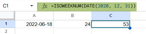
Step 3: Press Enter. You will see the ISO week number appear in cell B1 based on the date in A1. In this case, it returns 24, as 18th June 2022 was the 24th week according to the ISO calendar.

Step 4: You can try another familiar date. Here, we try =ISOWEEKNUM(DATE(2020, 12, 31)). As expected, we get 53, as it is the 53rd week according to ISO 8601.
Using the Google Menu Bar
You can also enter the number directly from the menu.
- Navigate to the menu bar at the top, then go to:
Insert ➝ Function ➝ Date ➝ ISOWEEKNUM - Select the function. Input the cell reference inside the parentheses of the formula.
- Press Enter, and the ISO week number will be calculated for the given date.
Examples
Let’s look at three detailed and practical examples that show the use of ISOWEEKNUM in real-time scenarios.
Example #1
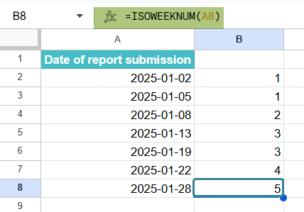
In this example, we have a list of daily reports submitted by employees. We wish to organize them by grouping them by the ISO week in which they were submitted.
Step 1: Enter all the dates in Column A.

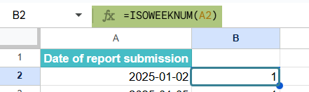
Step 2: In cell B2, enter the following formula:
=ISOWEEKNUM(A2)

Step 3: Press Enter. The result will show the ISO week number for that report date.
Step 4: Drag the formula down from B2 to all the rows containing dates. This allows you to see which ISO week each report falls under.
Example #2 – Using ISOWEEKNUM with IF Function
In this example, we want to find those tasks that were completed in ISO week 20 to calculate employee bonuses for that week. Let us look at how to do it with ISOWEEKNUM in Google Sheets. The function allows us to enter the values in a straightforward way.
Step 1: Enter all the details of the dates in Column A.

Step 2: In column B, let us use the following formula:
=ISOWEEKNUM(A2).
Drag the formula all the way down to B11 to get the ISO week number for all the dates.

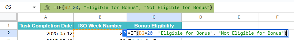
Step 3: Enter the following formula in C2.
=IF(B2=20, “Eligible for Bonus”, “Not Eligible for Bonus”)
This formula checks if the ISOWEEKNUM is the 20th week. If so, bonus is in the affirmative.
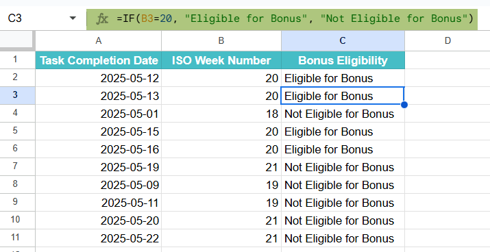
Step 4: Press Enter and copy the formula down. It will evaluate whether each date falls in week 20.
The result will return “Bonus Eligible” if the task was done during ISO week 20, and “Not Eligible” otherwise.
Example #3 – Using ISOWEEKNUM with Conditional Formatting
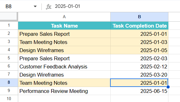
In another example, let us try to highlight all entries in a spreadsheet where the date belongs to ISO week 1. This helps in visually identifying the activities to be done at the beginning of a year. We can use the ISOWEEKNUM in Google Sheets directly in the conditional formatting section for this.
Step 1: Enter the details in columns A and B as shown below and select the range.

Step 2: Go to Format ➝ Conditional formatting. In the panel that appears, under Format cells if, choose Custom formula is. Enter the following formula:
=ISOWEEKNUM($B1)=1
Here, using $B1 ensures the formula applies correctly across rows, applying the formatting to both columns A and B.

Step 4: We have set a peach colored background above. Click Done.
All dates falling in the first ISO week of the year will now be automatically highlighted for easier reference.
Important Things to Note
- The ISOWEEKNUM function always considers Monday as the first day of the week.
- Also, remember that week 1 is defined based on the presence of January 4th, aligning with ISO 8601.
- If the input is not a valid date, the function will return a #VALUE error.
- The function does not consider time—only the date portion is used in the calculation.
Frequently Asked Questions (FAQs)
The main difference between WEEKNUM in Google Sheets and ISOWEEKNUM in Google Sheets is in how the weeks are defined. WEEKNUM allows customization of when a week starts (Sunday or Monday), but ISOWEEKNUM follows ISO 8601. Here, each week is considered to start on Monday and week 1 should contain January 4th. While WEEKNUM offers more flexibility in defining the start of the week, ISOWEEKNUM provides a standardized approach for consistent week calculations.
One can use a string-formatted date as long as it is in a recognizable format, and it will be considered a valid date. However, if the format is not standard or the string contains typos, the function will return an error. You can always use the DATE function to ensure that the date entered is in a valid format.
Most years contain 52 ISO weeks, but some can have 53 weeks depending on the year’s calendar layout. If January 1st falls on a Thursday or it’s a leap year that begins on a Wednesday, the year can include 53 ISO weeks. This ensures all days are covered well without overlap.
Use this ISOWEEKNUM in Google Sheets Template to follow along with the examples in this article.
Download Excel Template