
What Is COUNTIF Function In Google Sheets?
COUNTIF function in Google sheets is an inbuilt function used to count the data with specific criterions. It is a formula categorized under COUNT functions and as the name suggests, COUNTIF function counts the number of values or entries in the data with conditions. COUNTIF function in Google sheets helps users by counting specific entries. It is useful when we have to work with huge datasets.
For example, consider the below table showing names and marks in columns A and B respectively.
Use this COUNTIF Function In Google Sheets Template to follow along with the examples in this article.
Download Excel Template
Now, let us count the values with the data ‘Andy’ in the cell range.
To begin with, insert the data in the spreadsheet. In this example, the data is available in the cell range A1:B8. Now, select the cell where we want to insert the formula. In this example, it is cell B11. Next, insert the COUNTIF function formula in cell. So, the complete formula is =COUNTIF(A2:B8,A8). Press Enter key.
We will be able to see the result in cell as shown in the below image.

Likewise, we can use the COUNTIF formula in Google sheets.
In this article, let us learn more about COUNTIF function in Google sheets with detailed examples.
Key Takeaways
- COUNTIF function in Google sheets is a default function used to count the number of values with conditions.
- While working with huge datasets, we can use COUNTIF function to find values with specific entries.
- The syntax of COUNTIF function in Google sheets is =COUNTIF(range,criterion) where
- Range is the mandatory argument showing the cell range where we want to count the value
- Criterion is the condition with which we want to filter and count the value in the data.
- Remember, both the arguments are mandatory and we can use as many conditions we want with the formula.
COUNTIF() In Google Sheets Formula

The syntax of formula of COUNTIF function in Google sheets is =COUNTIF(range,criterion)
where
- Range is the cell range where we want to count the value
- Criterion is the condition or conditions with which we want to filter and count the value in the data.
- Both the arguments are mandatory.
How To Use COUNTIF Function In Google Sheets?
Let us learn how to use COUNTIF function in Google sheets with the help of the following steps.
Step 1: To begin with, insert the data in the spreadsheet. Now, select the cell where we want to insert the formula.
Step 2: Next, insert the COUNTIF function formula in cell.
Step 3: Press Enter key.
We will be able to see the result in the active cell.
Likewise, we can use the COUNTIF formula in Google sheets.
Examples
Now, let us learn how to use COUNTIF function in Google sheets with detailed examples.
Example #1 – Using Google Sheets COUNTIF To Count Non-Blank Cells
For example, consider the below table showing product and sales in columns A and B respectively.

Now, let us count the values with blank cells and non-blank cells in the cell range.
The steps are:
Step 1: To begin with, insert the data in the spreadsheet. In this example, the data is available in the cell range A1:B10. Now, select the cell where we want to insert the formula. In this example, we need to count non-blank cells in cell B13, and non-blank cells in cell B14.
Step 2: Next, insert the COUNTIF function formula in cell B13.

So, the complete formula is =COUNTIF(A2:A10,”<>”)
Step 3: Press Enter key.
We will be able to see the result in cell as shown in the below image.

Now, let us count the blank cells in cell B14.
The steps are:
Step 1: Select cell B14 and enter the COUNTIF formula in Google sheets.
So, the complete formula is =COUNTIF(A2:A10,””)

Step 3: Press Enter key.
We will be able to see the result in cell as shown in the below image.

Likewise, we can use the COUNTIF formula in Google sheets to count blank and non-blank cells.
Example #2 – Using Google Sheets To COUNTIF To Count Cells With Text And Numbers (Exact Match)
For example, consider the below table showing product and quantity (in Kg) in columns A and B respectively.

Now, let us count the values with the data ‘Apple’.
The steps are:
Step 1: To begin with, insert the data in the spreadsheet. In this example, the data is available in the cell range A1:B10. Now, select the cell where we want to insert the formula. In this example, it is cell B13.
Step 2: Next, insert the COUNTIF function formula in cell.
So, the complete formula is =COUNTIF(A2:B10,”Apple”)

Step 3: Press Enter key.
We will be able to see the result in cell as shown in the below image.

Likewise, we can use the COUNTIF formula in Google sheets.
Example #3 – Count In Google Sheets With Multiple Criteria – AND Logic
For example, consider the below table showing region, product and unit in columns A, B and C respectively.

Now, let us count the values with the data ‘North’ and ‘Laptop’ using AND Logic.
The steps are:
Step 1: To begin with, insert the data in the spreadsheet. In this example, the data is available in the cell range A1:C10. Now, select the cell where we want to insert the formula. In this example, it is cell C13.
Step 2: Next, insert the COUNTIF function formula in cell.
So, the complete formula is =COUNTIFS(A2:A10,”North”,B2:B10,”Laptop”)

Step 3: Press Enter key.
We will be able to see the result in cell as shown in the below image.

Likewise, we can use the COUNTIF formula in Google sheets with AND logic.
Example #4 – Count In Google Sheets With Multiple Criteria – OR Logic
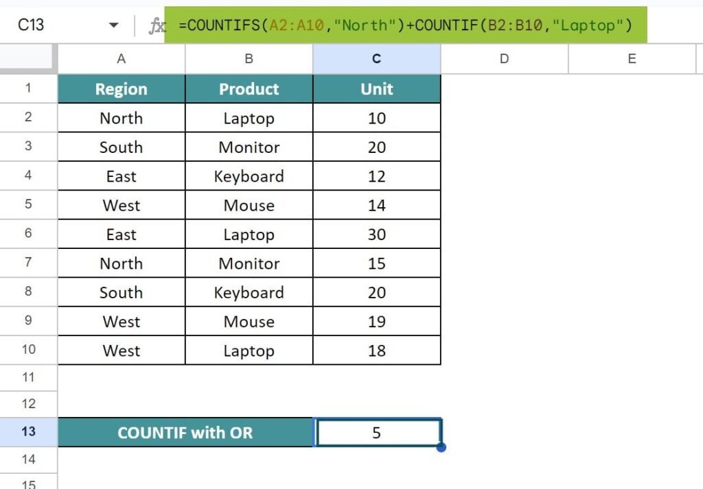
Now, let us use the same example we used in Example #3. Consider the below table showing region, product and unit in columns A, B and C respectively.

Now, let us count the values with the data ‘North’ and ‘Laptop’.
The steps are:
Step 1: To begin with, insert the data in the spreadsheet. In this example, the data is available in the cell range A1:C10. Now, select the cell where we want to insert the formula. In this example, it is cell C13.
Step 2: Next, insert the COUNTIF function formula in cell.
So, the complete formula is =COUNTIFS(A2:A10,”North”)+COUNTIF(B2:B10,”Laptop”)

Step 3: Press Enter key.
We will be able to see the result in cell as shown in the below image.
Likewise, we can use the COUNTIF formula in Google sheets with OR logic.
Important Things To Note
- COUNTIF function is a formula in Google sheets grouped under the COUNT functions.
- The COUNTIF function is used to count the values in the data with condition or criteria.
- We need to enter the correct logical operator to find the count of values with blank, non-blank, and blank with text data.
Frequently Asked Questions (FAQs)
For example, consider the below table showing subjects and the number of students in columns A and B respectively.
Now, let us count the values with the data ‘Physics’ in the given cell range.
The steps are:
Step 1: To begin with, insert the data in the spreadsheet. In this example, the data is available in the cell range A1:B8. Now, select the cell where we want to insert the formula. In this example, it is cell B11.
Step 2: Next, insert the COUNTIF function formula in cell.
So, the complete formula is =COUNTIF(A2:B8,”Physics”)
Step 3: Press Enter key.
We will be able to see the result in cell as shown in the below image.
Likewise, we can use the COUNTIF formula in Google sheets.
While using COUNTIF function in Google sheets, we can use the following logical operators.
They are:
• “<>” For non-blank cells
• “” for blank cells
• “*” for non-blank text values
COUNTIF Function in Google sheets may not work when we don’t include the correct cell range or logical operator. Users must remember to add the correct logical operator for blank or non-blank cells and also, to include ‘+’ or a comma to use the COUNTIF function with AND or OR function in Google sheets.
Use this COUNTIF Function In Google Sheets Template to follow along with the examples in this article.
Download Excel Template