
What Is SUMIF Text In Google Sheets?
The SUMIF Text in Google Sheets allows users to calculate the sum of values in a range based on specified criteria. Unlike the regular SUMIF function, which only accepts numerical values, the SUMIF Text function works with text or alphanumeric characters. It evaluates the cells in a given range and adds up only those cells that match the specified criteria.
The Google Sheets SUMIF Text function is particularly useful when dealing with data that contains both text and numbers, as it enables users to perform calculations based on specific text conditions.
Use this SUMIF Text In Google Sheets Template to follow along with the examples in this article.
Download Excel TemplateIn this example, we have the items and their quantities. We will use the SUMIF Text Google Sheets function to calculate the sum of the values that satisfy the criteria where the item names have the “G” letter.

Select cell D2, enter the formula =SUMIF(A2:A6,“*G*”, B2:B6) and press “Enter”.

The cells, A3 and A4, has the letter G, their corresponding values are taken into consideration and their sum is returned as 350.
Key Takeaways
- The SUMIF Text in Google Sheets is a conditional function that allows for the summation of cells based on specific criteria, including text. This powerful tool enables users to easily sum up a group of cells that meet a particular text-based condition.
- What sets this function apart is its indifference towards the case of the text, making it even more versatile and user-friendly. It also proves to be an invaluable asset for data analysis and calculation purposes.
- We can use this functions to find the exact or partial match, with single criterias such as, date or multiple criterias with criteria range, etc.
- Unlike SUMIFS, the SUMIF function cannot perform multiple criteria calculations. However, as a workaround, we can use the SUMIF multiple times and add the results or use the combination of the SUMPRODUCT and the SUMIF functions to perform multiple criteria calculations.
Syntax
The syntax of the SUMIF formula in Google Sheets is,

The arguments of the SUMIF formula in Google Sheets are,
- range – It is the values or range of cells that must be tested against the specified criteria. It is a mandatory argument.
- criterion – It is the criteria or the condition that will be checked against each value within the supplied range. It is a mandatory argument.
- [sum_range] – It is an optional argument. It allows us to specify the values or range of cells that should be added together if the “range” parameter meets the given condition or criteria. If this parameter is not provided, Google Sheets will automatically sum the cells specified in the range argument.
How To Use SUMIF Text In Google Sheets?
We can use the SUMIF Text function in Google Sheets in 2 ways, namely,
- Access from the Google Sheets ribbon.
- Enter in the worksheet manually.
Method #1 – Access from the Google Sheets ribbon –
Choose an empty cell for the output – select the “Insert” tab – click the “Function” option right arrow -click the “Math” option right arrow – select the “SUMIF” function, as shown below.

The “SUMIF” formulaappears, as shown below. Enter the argument as the cell reference.

Method #2 – Enter in the worksheet manually –
- Select an empty cell to display the output.
- Type = SUMIF( in the selected cell. Alternatively, type =S or =Sum and double-click the SUMIF function from the list of suggestions shown by Google Sheets.
- Enter the arguments as Google Sheets cell references or direct values.
- Close the parenthesis and press the Enter key.
Examples
Let us consider some examples to understand the SUMIF Text in Google Sheets w.r.t, exact match, partial match, blank or non-blank cells criteria and with multiple criterias with OR logic.
Example #1 – SUMIF with text criteria (Exact Match)
The below dataset consists of fruits and their price. We’ll be calculating the price of “Banana” in a given scenario.

The steps to find the exact match using the SUMIF Text are,
Step 1: Select cell D2 and enter the formula =SUMIF(A2:A8,“Banana”, B2:B8).

Step 2: Press “Enter”. We get the output as $100, because there is only one fruit matching the criteria “Banana”, as shown below.

Example #2 – SUMIF with wildcard characters (Partial Match)
Let’s consider the dataset of Example 1 to find the sum of the values of partial match of the criteria “Apple” using the wildcard character “asterisk = *”.

The steps to find the partial match using the SUMIF Text are,
Step 1: Select cell D2 and enter the formula =sumif(A2:A8,”*Apple”,B2:B8)

Step 2: Press “Enter”. We will get the output $1,050, as shown below. The criteria to check is for Apple and the cells A2, A4 and A7 has the word in their values. Therefore, the corresponding prices are totalled and returned as output.

Step 3: In cell D6, we will test the formula without the wildcard. So, the formula will be =sumif(A2:A8,”Apple”,B2:B8). The output is the exact match value, $500, as shown below.

Example #3 – SUMIF function with Date Criteria
In the following example, we have the dates and the sales of an XYZ company. We will calculate the sum of the values that satisfy the given date criteria, i.e., to calculate the sum till June sales.

The step to calculate the total using SUMIF for the given date criteria are,
Step 1: Select cell E2 and enter the formula = SUMIF(A2:A13,“ <=6/2/2023”,B2:B13).

Step 2: Press the Enter key. As a result, the sales till June, before the given date, i.e., 6/2/2023, are added and the result returned is $3,336,440, as shown below.

Example #4 – SUMIF Function With Blank or Not-Blank cells criteria
The below table data contains data of cities and the number of passengers as per the monthly statistics. We will calculate the total number of passengers with the criteria of blank or not blank cell values. We will perform the calculation using the SUMIF Text In Google Sheets for both the criterias city-wise and month-wise.

[Special Note:
- “<>” indicates “NOT EQUAL TO” sign à It has to be in double inverted commas as the formula processes it as characters. When we use this, the formula sums up all the values that are not blanks and completely ignores the blank cells during summation.
- “” indicates “Blanks” à Double inverted commas with no characters in them signify equal to blank. When we use this, it sums up all the values containing blanks and ignores cells containing some characters/values.]
The steps to perform the required calculation for blank and not-blank cells using the SUMIF function are as follows:
Step 1: First, let us calculate the city-wise passenger count.
- For not-blank cells, select cell F3, enter the formula =sumif(A2:A13,”<>”,C2:C13) and press “Enter”.
- For blank cells, select cell F4, enter the formula =sumif(A2:A13,””,C2:C13) and press “Enter”.
The output is shown below.

Step 2: Next, let us calculate the month-wise passenger count.
- For not-blank cells, select cell F8, enter the formula =sumif(B2:B13,”<>”,C2:C13) and press “Enter”.
- For blank cells, select cell F9, enter the formula =sumif(B2:B13,””,C2:C13) and press “Enter”.
The output is shown below. [Note: Column G is for our reference.]

Example #5 – SUMIF with multiple criteria (OR logic)
To handle multiple criteria, we have the SUMIFS function in Google Sheets. However, if want to use the SUMIF Text in Google Sheets, to sum numbers in one column when another column is equal to either A or B, we will see 2 methods or to perform SUMIF with multiple criteria.
Let us consider the example of the table given below which consists of the items and their sales. The requirement is to add up the sales for two different products, say Grapes and Oranges.

- Method 1: The most obvious solution is to handle each condition individually and then add their results: Therefore, the SUMIF with multiple criteria (OR logic) syntax will be as,
=SUMIF(range, criterion1, [sum_range]) + SUMIF(range, criterion2, [sum_range])
The procedure to calculate SUMIF for multiple criteria is,
Selectcell E4, enter the formula =SUMIF(A2:A10, “grapes”, B2:B10) + SUMIF(A2:A10, “oranges”, B2:B10) and press “Enter”.
[Note: We can also enter the criteria in separate cells and refer to those cells: Then the formula will be
=SUMIF(A2:A10, E2,B2:B10) + SUMIF(A2:A10, E3,B2:B10)
Where A2:A10 is the list of items (range), B2:B10 are the numbers to sum (sum_range), E2 and E3 are the target items (criteria) cell reference.]

The output is $945, as shown above. The first SUMIF totals the Grapes sales, the second SUMIF totals the Oranges sales and then, the addition operation adds the calculated totals of both the Grapes and Oranges and returns the output.
- Method 2: We can use the SUMPRODUCT and the SUMIF combination where the syntax will be as,
=SUMPRODUCT(SUMIF(range, criterion_range, [sum_range]))
The procedure to calculate using SUMPRODUCT and SUMIF for multiple criteria is,
Selectcell E4, enter the formula=SUMPRODUCT(SUMIF(A2:A10, E2:E3, B2:B10)) and press “Enter”.

The output is $945, as shown above. First, the SUMIF returns an array of numbers, representing the sums for each individual condition and then, the SUMPRODUCT adds these numbers.
Important Things To Note
- If there is an alpha-numeric or text values, then, the SUMIF ignores it and considers it as 0 and proceeds with the calculation.
- We must ensure to provide a valid “criterion”, else, the function will return the #VALUE! Error.
Frequently Asked Questions (FAQs)
We often forget in which category a function falls, here, the “SUMIF” function. Then, we can insert the function as follows:
Choose an empty cell – select the “Insert” tab – click the “Function” option right arrow – click the “All” option right arrow – select the “SUMIF” function, as shown below.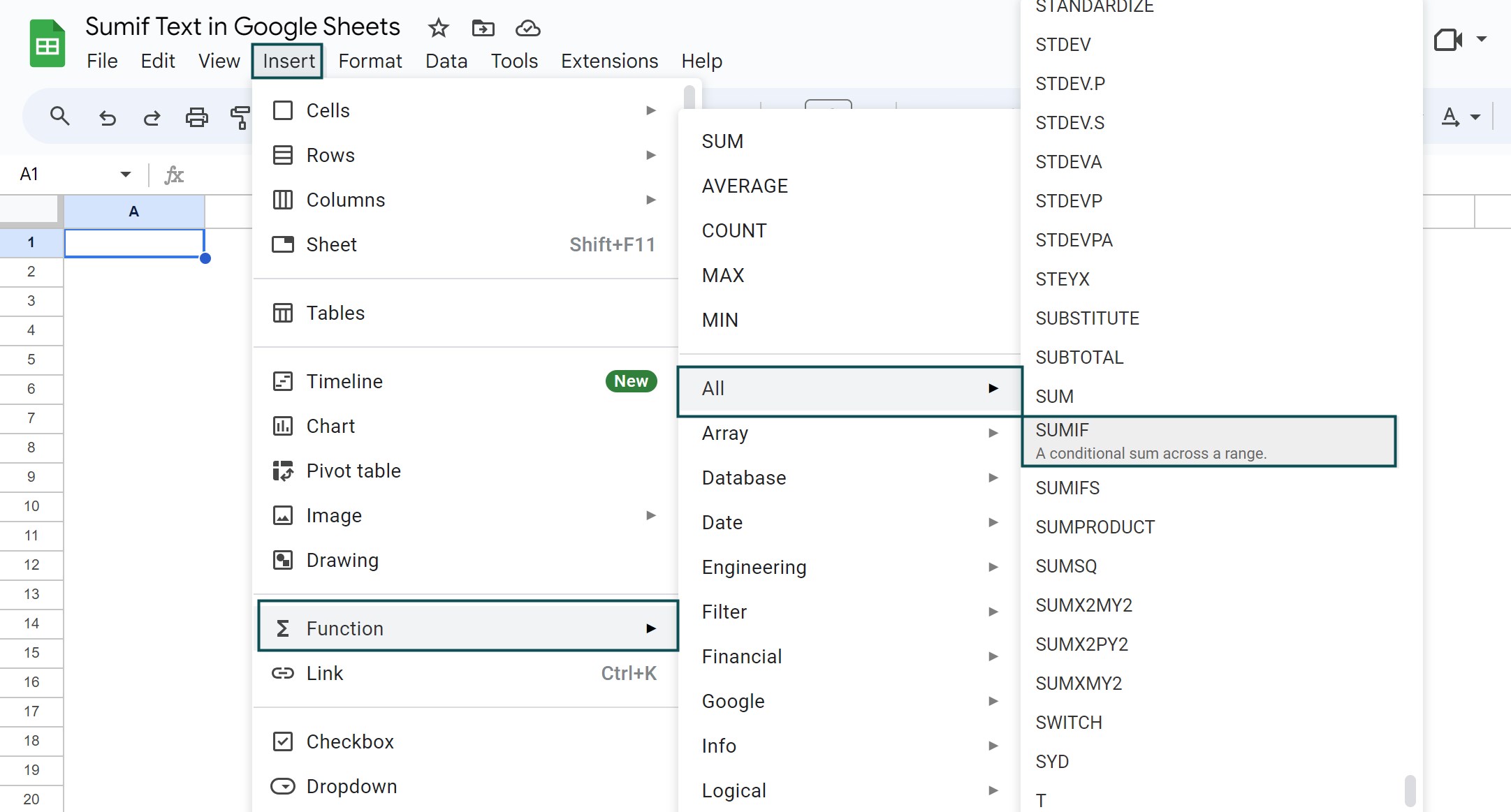
However, as always, entering the function manually is the best way to avoid confusion.
The SUMIF Text function, commonly used in Google Sheets, does not differentiate between uppercase and lowercase text. This function allows users to sum values in a range based on a specified criterion. However, when using the “text” criterion, it treats all text entries as case-insensitive. So, regardless of whether the text is uppercase or lowercase, the SUMIF Text function will consider.
The SUMIF function, typically used in spreadsheet software like Microsoft Excel or Google Sheets, allows users to sum a range of cells based on specified criteria. While SUMIF is a powerful tool for numerical criteria, it does have limitations when it comes to text criteria.
One limitation is that the function only supports partial matches with wildcards. For example, if “apple” is one of the text criteria, the function will not consider cells containing “apples” or “pineapple.”
Use this SUMIF Text In Google Sheets Template to follow along with the examples in this article.
Download Excel Template