
What is ISDATE in Google Sheets?
The ISDATE function in Google Sheets checks whether a value is a valid date. The function returns TRUE if the value is a date by Google Sheets, and FALSE if it is not. There are many such “IS” functions such as ISTEXT, ISNUMBER, and ISBLANK, and ISDATE is also helpful in validating the type of data entered in a cell. It helps ensure that the cell data is in a proper date format This can be important for calculations, filtering, or conditional formatting that is performed on dates.
For example, suppose we type 12/09/2025 in cell A1. To check if the entry is a valid date, enter the following formula in cell B1:
=ISDATE(A1)

The function will return TRUE since A1 contains a valid date. However, if the entry in not in a valid date format but contains text like 7th September, the formula would return FALSE because Google Sheets does not recognize it as a valid date. In this article, let us see how we can use the ISDATE function in Google Sheets. Let us have a glimpse at how it can validate dates in your spreadsheets, such that data integrity is maintained and errors can be prevented. This helps in managing projects, planning events, or generating financial reports.
Use this ISDATE in Google Sheets Template to follow along with the examples in this article.
Download Excel TemplateKey Takeaways
- The ISDATE function in Google Sheets checks whether a given value is a valid date. It returns TRUE if it is a date, and FALSE if not.
- The syntax of the ISDATE function is as follows: =ISDATE(value).
- It takes a single argument and evaluates whether the value entered is recognized as a date.
- One can combine ISDATE with other logical functions like IF, AND, OR to build more advanced validation rules.
- Since dates in Google Sheets are stored as serial numbers, valid date entries may also return TRUE when tested with ISNUMBER.
Syntax
The formula of ISDATE in Google Sheets is as follows:
=ISDATE(value)
value: (mandatory) It is the value that you want to check for a valid date. It can be a date, a reference value, a blank value or a text/number.
How To Use ISDATE Function in Google Sheets?
The function takes a single argument: =ISDATE(value). Hence, it is simple and straight-forward to use. We can use the ISDATE function in Google Sheets in two ways:
- By typing it directly into a cell.
- By accessing it from the Google Sheets menu bar.
Let us go through both methods step by step.
Entering ISDATE in Google Sheets Manually
The steps to type the ISDATE function manually in a cell are as follows:
Step 1: Consider a case where we have some values in cells A2 to A4 in Google Sheets. We want to verify if these values are valid dates.

Step 2: In cell B2, start by typing the function name and opening the parentheses.
=ISDATE(
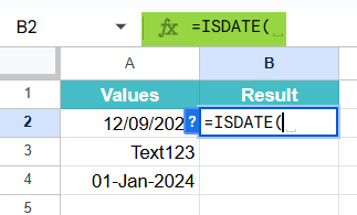
Next, provide the cell reference that you want to check. In this example, it is A2. Close the parentheses to complete the formula. Press Enter to see the output in cell B2.

Step 3: Drag the formula down to cell B4 so that all the values are checked. The function will return TRUE if the entry is a valid date and FALSE if not.

Using ISDATE Through the Menu Bar
Another way to use ISDATE is from the menu bar. Here’s how:
- Click on the cell where you want the result to appear.
- Go to Insert -> Function -> Info.
- From the list, choose ISDATE.
- Enter the required argument inside the parentheses.
- Press Enter.
Examples
Let’s look at some examples to see how the ISDATE function works in action. These will help you quickly understand how the function returns TRUE for valid dates and FALSE for everything else.
Example #1
A company has a list of entries submitted by employees as their joining dates. Some of them have entered actual dates, while others might have made mistakes in their typing like text. We must verify which entries are valid dates and which are not using the ISDATE function. Here, we will apply the ISDATE function to check each entry in column B and confirm whether it is a valid date or not.
Step 1: Enter the details in a table as shown below. In cell C2, type the following formula:
=ISDATE(B2)
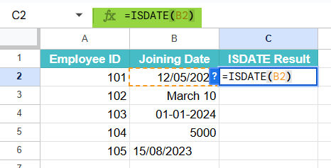
Step 2: Press Enter to see the result for the first value.

Step 3: Drag the formula down from cell C2 to C6 so that it applies to all rows.
Check the results. TRUE will appear if the entry is a valid date, and FALSE will appear if it is not recognized as a date.

The final entry is FALSE because you can the that the date entered is actually a text from the way it is aligned away from the other values.
Thus, the ISDATE function quickly identifies valid date entries and flags incorrect data types. This makes it easier to clean information before using it in further analysis.
Example #2 – Using ISDATE with Conditional Formatting
There is a list of project deadlines submitted by different team members. Some of them have entered proper dates, while others mistakenly typed text values or left the cell blank. To quickly highlight the cells that contain valid dates, we can use the ISDATE function with conditional formatting.
Step 1: Select the range of cells that contains the project deadlines. It is entered in a sheet.

Step 2: From the menu, go to Format -> Conditional formatting.

Step 3: In the conditional format rules pane, under Format cells if…, choose Custom formula is.
Enter the formula:
=ISDATE(B2)

Step 4: Choose a formatting style, such as a blue fill color, to highlight all valid dates. Click Done.

Now, all cells that contain valid dates will automatically be highlighted, while invalid entries like text or numbers will remain unformatted. This method is very useful when reviewing large datasets, as it helps you quickly spot valid deadlines and identify incorrect or missing entries.
Example #3 – Using ISDATE to Validate a Data Range
Some employees of a company are on leave and submitting applications where each person must enter a start date and end date. However, some accidentally type text like “Next Friday” or leave cells empty instead of entering proper dates. We can use the ISDATE function to validate the data range.
Step 1: Let us look at how the employees have entered the details in a sheet.

Step 2: In cell C2, enter the following formula to check if the “Leave Start Date” in cell A2 is valid:
=ISDATE(A2)

Step 3: Press Enter. If the value is a valid date, the result will be TRUE. Otherwise, it will show FALSE.
Copy the formula to column D to check the “Leave End Date” for each employee. Here, the formula becomes =ISDATE(B2).

Step 4: Drag both formulas down to validate the entire list of entries.

With this approach, you can immediately identify which rows contain incorrect date entries and quickly follow up to correct them. This ensures that all the data in your leave tracker is clean and usable for further processing.
Important Things to Note
- If a value is not in a format recognized as a date, ISDATE will return FALSE.
- When providing a date directly within the ISDATE formula, it must be enclosed in quotation marks (e.g., =ISDATE(“1/1/2025”)).
- ISDATE only checks if a value is formatted as a date; it does not validate the logical correctness of the date itself (e.g., it won’t flag “February 30th” as invalid
- ISDATE is particularly useful for data validation, conditional formatting (e.g., highlighting invalid date entries), and filtering data based on whether a cell contains a date.
Frequently Asked Questions (FAQs)
One of the biggest challenges when working with dates is dealing with many date formats. Different firms or regions use different date formats, such as MM/DD/YYYY or DD/MM/YYYY. However, Google Sheets can handle multiple formats, but it should be consistent across the range or sheet to avoid discrepancies.
Everyone using the sheet to adhere to a fixed format by going to the Format menu, and choosing “Number” and then “Date.”
Sometimes, values that look like dates are stored as text in Google Sheets. For example, when we type “2025/09/08” with spaces and it gets formatted as text, Google Sheets treats it as text. To fix this, re-enter the value or change the cell format to “Date.”
ISDATE verifies whether the value is a valid date, while ISTEXT checks if the value is a plain text. For example, “01/01/2025” will return TRUE for ISDATE if it is a valid date but FALSE for ISTEXT. On the other hand, “January 1, 2025” typed as text will show TRUE for ISTEXT but FALSE for ISDATE.
One can combine ISDATE with IF to display custom messages instead of TRUE or FALSE. For example:
=IF(ISDATE(A1),”Valid Date”, “Invalid Entry”)
Gives “Valid Date” if the function is TRUE, and “Invalid Entry” if the function is FALSE.
Use this ISDATE in Google Sheets Template to follow along with the examples in this article.
Download Excel Template