ISNUMBER In Google Sheets

What Is ISNUMBER Function In Google Sheets?

The ISNUMBER in Google Sheets checks the selected cell values in a dataset and returns “TRUE” if the cell value is a number or else “FALSE” if there are any other values found.

With the help of conditional functions, we can use the Google Sheets ISNUMBER function to return alternate values, other than the default TRUE or FALSE.

For example, we have some random values in the table below. Let us check for numeric cells using the ISNUMBER function in Google Sheets.

Select cell B2, enter the formula =ISNUMBER(A2), press “Enter” and drag the formula from cell B2 to B6 using the fill handle, as shown below.

ISNUMBER in Google Sheets Definition 1-1

The output is shown above, i.e., the ISNUMBERformula returned “TRUE” for the numeric values cells regardless of whether it is an amount, contact number, integer, etc, and “FALSE” if the cell values are non-numeric.

The ISNUMBER in Google Sheets is an Information function, that check the selected dataset exclusively for numeric cells. The return value is always the logical values, “TRUE” or “FALSE”, whether the searched cell value is a number or not, respectively.
It is a single argument function, i.e., we can select only one cell at a time and drag the formula for the rest of the cells. However, to select a cell range we can execute the formula as an array formula by selecting the keys “Ctrl+Shift+Enter”.
To get alternate or spiced up results other than the default “TRUE” or “FALSE”, we can insert the IF function condition in the ISNUMBER formula.
We can select a cell range when we need to apply the “Conditional Formatting” to the dataset and insert the ISNUMBER formula.

Syntax

The syntax of the ISNUMBER Formula in Google Sheets is,

The one and only mandatory argument of the ISNUMBER Formula in Google Sheets is,

value – It is the selected cell to check whether it is a numeric value or not.

How To Use ISNUMBER Function In Google Sheets?

We can use the ISNUMBER Google Sheets Function in two ways, as follows:

Access from the Google Sheets ribbon.
Enter the formula in the worksheet manually.

Method #1 – Access From the Google Sheets Ribbon

Step 1: Choose an empty cell for the output à select the “Insert” tab à click the “Function” option right arrow à click the “Info” option right arrow à select the “ISNUMBER” function, as shown below.

Step 2: The “ISNUMBER” formulaappears, as shown below. Enter the argument as cell reference.

Method #2 – Enter the Formula in the Worksheet Manually

Step 1: Select an empty cell for the output.

Step 2: Type =ISNUMBER( in the cell, as shown below. [Alternatively, type =IS or =ISN and double-click the ISNUMBER function from the Google Sheets suggestions.]

Step 3: Enter the arguments as cell values or cell references and close the brackets.

Step 4: Press Enter to view the outcome.

Examples

We will understand the function using the ISNUMBER in Google Sheets examples.

Example #1 – ISNUMBER on an Array of Cells.

The data table given below consists of smartphones quarterly sales, where the data entered are all sales, i.e. the numeric values. Now, we will use the ISNUMBER on an array of cells and get the results.

We have also created a result table with the same headers and have copy only the formatting and not the values, because we must execute the ISNUMBER() as an array. It helps us view the result cells in a better way.

The steps to use ISNUMBER on an array of cells are,

Step 1: Select cell B10 and enter the formula =ISNUMBER(B2:D7), as shown below.

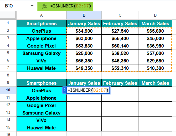
ISNUMBER on an array of cells Example 1-1

Step 2: Since we are executing as an array formula,press the “Ctrl+Shift+Enter” keys and then press “Enter”. Now the formula looks like this =ArrayFormula(ISNUMBER(B2:D7))

ISNUMBER on an array of cells Example 1-2

The output is shown above. The moment we press “Enter”, all the result cell range gets populated as “TRUE”, because the sales amount are all numeric values regardless of the currency.

Example #2 – Using ISNUMBER in Data Validation.

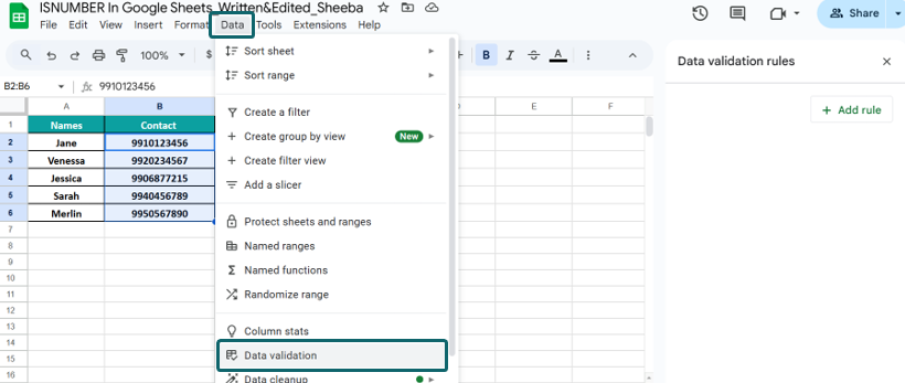
The data given below consists of user’s names, their contact numbers and email ids. We will Using ISNUMBER in Data Validation and ensure to leave the numeric cells as it is, meaning, the rule set will not allow non-numeric data to be added to the numeric cells or the data validation applied cells.

Using ISNUMBER in Data Validation Example 2

The steps to use ISNUMBER in Data Validation are as follows:

Step 1: Choose cell B2:B6 à select the “Data” tab à click the “Data validation” option and the “Data validation rules” window appears on the right, as shown below. Here, click the “Add rule” button.

Using ISNUMBER in Data Validation Example 2-1

Step 2:

Choose the “Custom formula is” option from the “Criteria” drop-down and enter the formula “=ISNUMBER(B4)” in the field that appears below.
Next, choose the “Reject the input” option from the “If the data is invalid:” option.
Finally, click the “Done” option, as shown below.

Using ISNUMBER in Data Validation Example 2-2

Step 3: Now to check the rule, let us try to enter non-numeric value in cell B4, here abc.

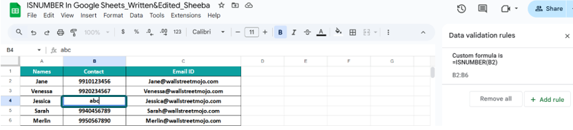
Using ISNUMBER in Data Validation Example 2-3

Immediately, we get an error, as shown below.

Using ISNUMBER in Data Validation Example 2-4

Therefore, as per the set rule, the cells B2:B6 must always be a numeric value cell and does not accept any other non-numeric input.

Example #3 – Combining ISNUMBER and SEARCH Functions.

Consider the dataset that consists of some strings and the substring of the same. We will find if the searched value is a number or not by Combining ISNUMBER and SEARCH Functions. In column C we have executed the SEARCH formula result for our reference.

[Note: The SEARCH Function returns the position or index value of a specified substring within a text string].

Combining ISNUMBER and SEARCH Functions 1

The steps to detect the numeric value in the SEARCH result cells are,

Step 1: Select cell D2, enter the formula, =ISNUMBER(SEARCH(B2,A2)) and press “Enter”, as shown below.

Combining ISNUMBER and SEARCH Functions 1-1

Step 2: Drag the formula from cells D2 to D4 using the fill handle, to get the following results.

Combining ISNUMBER and SEARCH Functions 1-2

The output is shown above. If the SEARCH results are a number, or the position of the substring searched for, then the formula returns “TRUE”. Else, the output as “FALSE” as seen in cell D3, because the result of the SEARCH formula is an error and not a number.

Example #4 – ISNUMBER with Conditional Formatting.

The dataset given below has the marks scored by a student in an exam. Let us highlight the numeric values using the ISNUMBER with Conditional Formatting.

The steps to use the ISNUMBER() function to apply the Conditional Formatting feature are as follows:

Step 1: First, choose the cell range A1:C9 à select the “Format” tab à click the “Conditional formatting” option. The “Conditional format rules” pane appears on the right side. There, click the “Add another rule” option, as shown below.

ISNUMBER with Conditional Formatting 1-1

Step 2:

We see the “Single Color” and the “Color scale” tabs. Here, click the “Single color” tab, select the “Custom formula is” option from the “Format cells if…” drop-down, as shown below.
When we select the “Custom formula is” option, an empty field appears below. There, enter the formula =ISNUMBER(A1) and select the required color, here, cyan, from the “Formatting style” options.
Finally, click the “Done” option, as shown below.

ISNUMBER with Conditional Formatting 1-2

We get the output shown below, where only the numeric cells are highlighted.

ISNUMBER with Conditional Formatting 1-3

Important Things To Note

The ISNUMBER function can only be applied to a single cell. We will get the result as “False” if we select multiple values or a cell range as arguments, unlike MS Excel, where we get an error message as, “You’ve entered too many arguments for this function.”.
The ISNUMBER function can be combined with other functions like the IF function to get alternate results other than the default, TRUE or FALSE.

Frequently Asked Questions (FAQs)

1) What is an alternate way to insert the ISNUMBER in Google Sheets?

We often forget in which category a function falls, here, the “ISNUMBER” function. Then, we can insert the function as follows:

Choose an empty cell → select the “Insert” tab → click the “Function” option right arrow → click the “All” option right arrow → select the “ISNUMBER” function, as shown below.

However, as always, entering the function manually is the best way to avoid confusion.

2) Where else can we find the ISNUMBER function in Google Sheets?

Alternatively, we can find the Functions icon to insert the ISNUMBER function in Google Sheets by following the path shown below.

• Choose an empty cell → click the “More” option represented by the three vertical dots at the end of the toolbar, as shown below.

• A list of icons appears when we click the “More” option. Here, click the “Functions” icon.

• Here, click the “Functions” option → click the “All” option right arrow → select the “ISNUMBER” function, as shown below.

3) Why is the ISNUMBER in Google Sheets not working?

The ISNUMBER in Google Sheets may not work due to the following reasons:

• The ISNUMBER in Excel may return “False” even though the result cell is a number. The function may not recognize the number because the formatting may be text. In such cases we can align the numeric values or check the formatting.
• We have provided the cell range instead of a single cell reference, as the argument value.
• The cell value is provided directly in the formula and is entered within double-quotes. Therefore, the value is mistaken for a text value. For example, =ISNUMBER(“123”).

Download Template

This article must help understand ISNUMBER in Google Sheets with its formula and examples. You can download the template here to use it instantly.

ISNUMBER Function In Google Sheets Excel Template Download

ISNUMBER In Google Sheets