
What is ARRAYFORMULA in Google Sheets?
The ARRAYFORMULA in Google sheets is used to perform calculations on an entire range of cells simultaneously instead of a single cell. Normally, the regular formulas work only on individual cells. However, when we use ARRAYFORMULA, we can apply the function to multiple cells at once. This is very useful when you wish to avoid dragging formulas down a column manually. It can work for operations like mathematical calculations, logical comparisons, and text manipulations across ranges.
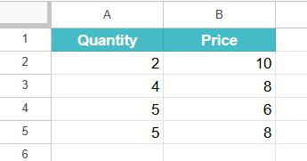
For example, here we will multiply values in column A with values in column B and display the result in column C. Instead of writing =A1*B1 and copying it down, you can simply use the formula below in cell C1:
Use this ARRAYFORMULA in Google Sheets Template to follow along with the examples in this article.
Download Excel Template=ARRAYFORMULA(A1:A * B1:B)
This will automatically apply the multiplication to each corresponding pair of cells in columns A and B and return the results in column C.

Key Takeaways
- The ARRAYFORMULA function lets you apply a formula to an entire range of cells using a single formula without the need to drag down.
- The syntax of the function is as follows:
=ARRAYFORMULA(array_formula)- array_formula: A formula or expression that works across ranges instead of individual cells.
- ARRAYFORMULA works well with functions like IF, LEN, and TEXT to process entire columns simultaneously.
- If the output range includes non-empty or merged cells, ARRAYFORMULA will return a #REF! error.
- To make the formula update with new data automatically, use open-ended ranges like A2:A instead of fixed ones like A2:A10.
Syntax
The syntax of ARRAYFORMULA in Google Sheets is:
=ARRAYFORMULA(array_formula)
- “array_formula,” refers to a mathematical expression, range, or function that returns multiple results you want to apply across multiple cells.
- One can process multiple values instead of a single value, thereby helping perform dynamic calculations across rows or columns without manually copying or dragging formulas.
The ARRAYFORMULA is especially useful when working with large datasets or when you want to apply the same operation to an entire column.
How To Use ARRAYFORMULA Function in Google Sheets?
ARRAYFORMULA in Google Sheets is very useful in scenarios where you do not wish to copy-paste the formula to an entire range of cells at once, eliminating the need to copy it down manually.
There are two main ways to use the ARRAYFORMULA function in Google Sheets:
- Enter the function manually.
- Through the Google toolbar
Enter the Function Manually
Using ARRAYFORMULA is powerful and saves you time, especially when working with large data ranges. One can apply formulas to entire columns without needing to copy them down manually.
Step 1: Open a new sheet and enter the data in two columns.
Step 2: Select the cell where you want the result of the ARRAYFORMULA to appear (e.g., C1). Go to the cell.
Step 3: Now, enter the formula as shown below. Start with an = sign, followed by the function name and opening braces.
Next, enter the arguments as shown below, separated by a comma.
Close the parentheses.
=ARRAYFORMULA(A2:A5 * B2:B5)
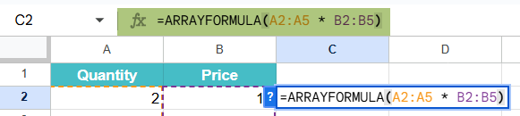
This formula multiplies the values in column A by those in column B row by row. You get the result simultaneously as shown below.
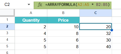
Step 4: Press Enter. Google Sheets will automatically display the results for all rows within the specified range in column C.
Through the Google toolbar
- Choose the cell where you want to apply the ARRAYFORMULA.
- Go to the menu bar and click on “Insert” ➝ “Function” ➝ “Array” ➝ “ARRAYFORMULA”.
- Google Sheets will insert the function. You can enter your range or formula inside the brackets. Press the Enter key. The results will appear instantly across the range.
Examples
Let us look at some ARRAYFORMULA examples to understand clearly the ways in which one can use it to apply formulas across ranges. It is especially useful for performing operations like row-wise multiplication, conditional logic, etc., without manually dragging the formula.
Example #1
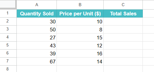
In this example, a store has a list of products with their total quantity sold and price per unit. The normal way is to multiply each row manually. Let us use ARRAYFORMULA to calculate the total sales for each item in one go without dragging down the formula.
We’ll use the ARRAYFORMULA function to multiply the values in column A and column B.
Step 1: In a new sheet, enter the data. Here, we enter the quantity sold in Column A and the price per unit in Column B.
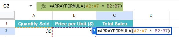
Step 2: Select the cell C2 where you want the total sales to appear.
Type the following formula in it.
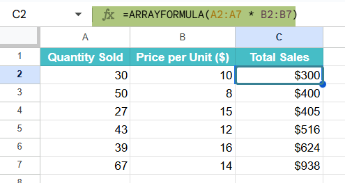
=ARRAYFORMULA(A2:A7 * B2:B7)
This multiplies each value in A2:A5 by its corresponding value in B2:B5.
Step 4: Press Enter. The formula will automatically calculate all the totals in column C without needing to drag the formula down manually.
Example #2 – Combining ARRAYFORMULA with IF Function
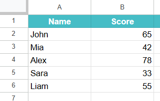
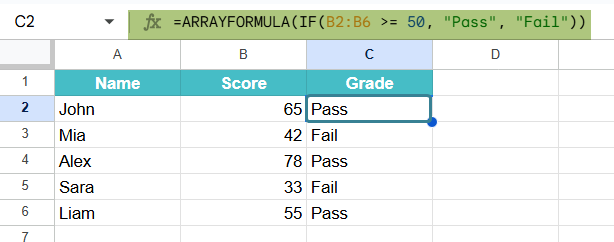
A teacher at a school has a list of student scores. They wish to assign Pass or Fail to each student based on their score. Here, scores >= 50 are considered Pass and marks below that threshold are considered as Fail.
Instead of writing an IF formula for every row, we’ll use ARRAYFORMULA with IF to evaluate all student scores at once and assign grades in a single formula.
Step 1: As shown below, enter the student names in column A and their scores in column B.
Step 2: Click on cell C2, where we wish the grades (Pass/Fail) to appear, and type the following formula:
=ARRAYFORMULA(IF(B2:B6 >= 50, “Pass”, “Fail”))
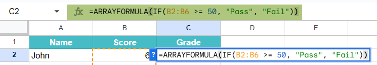
This formula checks each score in column B. If it is 50 or more, it returns “Pass”; otherwise, it returns “Fail”.
Step 4: Press Enter. Google Sheets will instantly apply the logic to all rows in the range, displaying the result in column C without needing to drag the formula.
Example #3 – Combining ARRAYFORMULA with COUNT
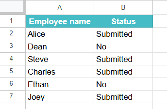
A manager of a team is tracking who has submitted their weekly reports. He has a list of employee names and their report submission status. Some cells in column B are filled (meaning the report was submitted), while others are blank (not submitted).
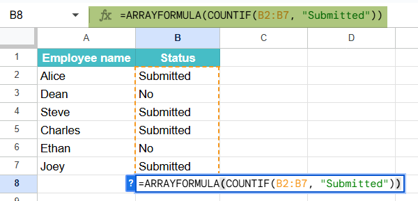
The manager must automatically count how many team members submitted their reports using ARRAYFORMULA with the COUNT logic. Let us look at how to do the same.
Step 1: We enter employee names in column A and their submission status in column B.
Step 2: Click on cell C2 where you want the total count of submitted reports to appear and enter the following formula:
=ARRAYFORMULA(COUNTIF(B2:B7, “Submitted”))
This counts how many times the value “Submitted” appears in the range B2:B7 using COUNTIF. ARRAYFORMULA ensures it’s applied to do it on one go.
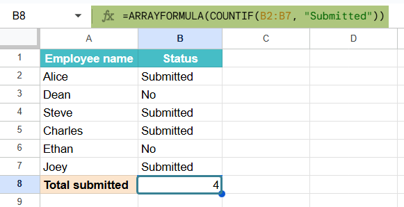
Step 4: Press Enter. The result will show the count of all employees who submitted their reports.
Important Points to Note
- ARRAYFORMULA works best with functions that are compatible with arrays, such as IF, LEN, ISBLANK, TEXT, etc.
- Unlike other drag-down formulas, ARRAYFORMULA automatically updates as new rows are added if the referenced range is open-ended (e.g., B2:B). Thus, this formula is ideal for dynamic data.
- All columns or ranges in the formula must be the same size, or it may show an error.
Frequently Asked Questions (FAQs)
Here are scenarios that cause a #REF! error when using ARRAYFORMULA in Google Sheets.
1. Overlapping Output: The formula tries to place values in cells that already contain data. Always ensure the output range is empty.
2. Merged Cells in Output Range: If the output range includes merged cells, we get the error.
3. Mismatched Range Sizes: If we combine multiple ranges with different sizes(like A2:A5 and B2:B7), it may result in this error.
4. Some functions like ARRAYFORMULA(VLOOKUP Google Sheets) don’t work well and can also result in #REF!.
ARRAYFORMULA works well with many functions, and we list some of them below
1. IF – it can be used to apply conditions across a range.
Example: =ARRAYFORMULA(IF(B2:B6 >= 50, “Pass”, “Fail”))
2. LEN – It can count the number of characters in each cell of a column.
Example: =ARRAYFORMULA(COUNT(A2:A6))
3. TEXT – This will format dates or numbers across multiple rows at once.
Example: =ARRAYFORMULA(TEXT(C2:C6, “MM/DD/YYYY”))
This makes it easy to process data row-by-row using just one formula.
It can update automatically when we use open-ended ranges like A2:A instead of fixed ranges like A2:A10. This allows the formula to automatically include new data as one adds more rows, making it very useful for increasing datasets.
Use this ARRAYFORMULA in Google Sheets Template to follow along with the examples in this article.
Download Excel TemplateRecommended Articles
Continue with these related resources when you want the next practical step in this topic.
- LAMBDA in Google Sheets
- VSTACK in Google Sheets
- CHOOSECOLS in Google Sheets
- HSTACK in Google Sheets
- LET in Google Sheets
Explore the full Google Sheets Dynamic Arrays and Advanced Functions guide or browse Google Sheets Resources.