CHOOSECOLS in Google Sheets

What is CHOOSECOLS in Google Sheets?

CHOOSECOLS in Google Sheets is a function that allows users to extract specific columns from a given range or array based on their index numbers. This function is particularly useful for dynamically selecting and displaying certain columns without manually copying, pasting, or filtering. The primary purpose of CHOOSECOLS is to simplify data management and analysis by enabling the quick extraction of relevant columns for reports, dashboards, or focused analysis, without modifying the original dataset.

For example, input this formula in an empty cell to get the columns from the entered data.

=CHOOSECOLS(A1:B6, 1). You will get the 1st column from the range A1:B6 displayed in the selected area.

Syntax

The formula for CHOOSECOLS is straightforward:

=CHOOSECOLS(array, col_num1, [col_num2, …])

• array: This is the range or array from which you want to extract columns.
• col_num1, [col_num2, …]: These are the index numbers of the columns you want to select from the array. Column counting starts at 1, which is the first column of the specified array. You can specify multiple columns, including non-contiguous ones, and even repeat column numbers to display the same column multiple times.

How to Use CHOOSECOLS Function in Google Sheets?

The CHOOSECOLS function is used to return specific columns from a range based on their position. It is useful when you want to select only certain columns for analysis, create reports, or display relevant data without manually copying or hiding columns.

To enter CHOOSECOLS in Google Sheets, there are two main ways:

• Enter CHOOSECOLS manually
• From the Google Sheets menu

Enter CHOOSECOLS Manually

To use CHOOSECOLS in Google Sheets manually, follow this simple example:

Step 1: Create a table with column headers. For example, a table with Student ID, Name, and Grade.

Step 2: Click on the cell where you want the result to appear. Type =CHOOSECOLS(

=CHOOSECOLS(

Step 3: Enter the array (your data range) and the column numbers you want to return. You can specify one or multiple columns.

=CHOOSECOLS(A2:C6, 2, 3)

Here, we are selecting the 2nd column and 3rd column.

Step 4: Press Enter. The function will return only the columns you selected.

In this example, we manually entered the CHOOSECOLS formula in a cell and specified which columns to extract from our table. This method shows how you can dynamically display only the columns you need, making data analysis and reporting faster and more efficient.

Entering CHOOSECOLS Through the Menu Bar

1. Go to the Insert tab. Choose Function -> Lookup.
2. From the list, select CHOOSECOLS.
3. Fill in the proper cell ranges and column positions.
4. Press Enter to get the result.

Thus, you can extract specific columns from your dataset easily without manually hiding or copying them.

Examples

The primary purpose of CHOOSECOLS is to allow users to select and return specific columns from a specified range. Imagine having a large dataset with multiple fields, but you only need a few key pieces of information for your report or analysis. Instead of manually hiding or copying columns, CHOOSECOLS lets you extract the exact columns you need quickly and efficiently. Let us look at some CHOOSECOLS in Google Sheets examples.

Example #1

Suppose you have a table of students with multiple subjects and grades, and you only want to display the Name and Maths columns for reporting purposes. The CHOOSECOLS function can pull only the required columns without altering the original dataset.

Step 1: Set up your table with the following headers: Name, Maths, Science, English, and Total. Fill in data as shown in the table below.

Step 2: Click on an empty cell where you want the extracted columns to appear. Type the following formula:

=CHOOSECOLS(A2:E6, 1, 2)

• A2:E6 is the range containing the full dataset.
• 1, 2 are the column positions within that range you want to extract (Name and Maths).

Step 3: Press Enter. The function will return only the selected columns from the original dataset, keeping the data dynamic—if the source table changes, the result updates automatically.

By using CHOOSECOLS, we efficiently extracted only the relevant columns for analysis without manually hiding or copying the other data. This is particularly useful for reporting or creating dashboards from larger datasets.

Example #2 – Using CHOOSECOLS to extract the First and Last Rows

One of the unique features of CHOOSECOLS is its ability to return columns from both the beginning and the end of a dataset. When working with large spreadsheets, you can instantly extract the first and last columns without manually hiding or deleting other columns. This is especially useful when you want to display key identifiers and final results together, such as Student Name and Total Score in a grading sheet.

Step 1: Set up the table as shown below. Here, again we have a list of students and their scores in multiple subjects, along with the total score.

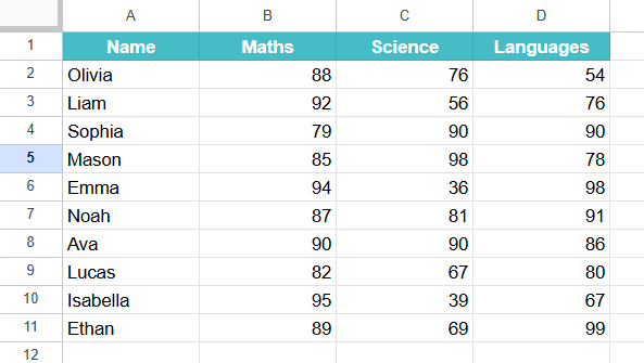
Step 2: Click on the cell where you want the result to appear. Type the following formula:

=CHOOSECOLS(A2:D11, 1, -1)

Here:

• A2:D11 is the range.
• 1 extracts the first column (ID).
• -1 extracts the last column (Total). Negative numbers count from the end of the range.

Step 3: Press Enter. The function will return only the first and last columns from the dataset.

You can quickly display both the first and last columns in a dataset using CHOOSECOLS. This feature saves time when tracking identifiers alongside final results, totals, or summary metrics in large spreadsheets.

Example #3 – Using CHOOSECOLS with ARRAYFORMULA Function

While CHOOSECOLS works well for extracting specific columns by position, sometimes you may want to first filter or dynamically manage the dataset and then select certain columns from that output. By combining ARRAYFORMULA with CHOOSECOLS, you can handle expanding datasets without manually adjusting ranges.

Step 1: Enter all the required details as shown below. In this example, we have a small dataset of employees with their Name, Department, Age, and Salary.

Step 2: Suppose we only want to extract the Name and Salary columns, and we want the formula to automatically adjust when new employees are added. Enter the following formula:

=ARRAYFORMULA(CHOOSECOLS(A2:D100, 1, 4))

Here:

• A2:D6 is the range of the dataset.
• 1, 4 extracts the first column (Name) and last column (Salary).

ARRAYFORMULA ensures the formula dynamically expands when more rows are added.

Step 3: Press Enter. The output will automatically show the selected columns for all existing employees.

Step 4: The table will expand if new entries are added to the dataset because we have used ARRAYFORMULA.

By combining ARRAYFORMULA with CHOOSECOLS, you can dynamically extract non-contiguous columns from a dataset that may grow over time. This approach is particularly useful for automated reports, dashboards, and real-time analysis, as it eliminates the need to manually update formulas whenever new data is added.

Important Things To Note

1. Negative column numbers count from the end, so -1 selects the last column dynamically.
2. Non-contiguous columns can be repeated or reordered, such as =CHOOSECOLS(A2:F10, 3, 1, 3).
3. Combining CHOOSECOLS with ARRAYFORMULA allows automatic updates when new columns or rows are added.
4. You can use cell references instead of hardcoding column numbers, e.g., =CHOOSECOLS(A2:F10, G1).
5. It creates a new array without altering the original dataset, which can be used in further calculations or charts.

Frequently Asked Questions (FAQs)

Download Template

This article must help understand CHOOSECOLS Function in Google Sheets with its formulas and examples. You can download the template here to use it instantly.

Recommended Articles

Guide to What is CHOOSECOLS Function in Google Sheets. We learn how to use CHOOSECOLS function in Google Sheets with its syntax and examples. You can learn more from the following articles. –

NPV in Google Sheets

CUMIPMT in Google Sheets

DPRODUCT in Google Sheets