
What is DPRODUCT in Google Sheets?
The DPRODUCT function in Google Sheets can multiply the values in a given numeric field in a table that matches some given conditions. The function returns the product of values selected from the database or range using a query similar to SQL.
It is not a very commonly used function in Google Sheets. Nevertheless, it is a very useful function for performing conditional product calculations in structured datasets. As an example, if there is a list of products with their Quantity and Price in a table, and we have to calculate the product of prices for those items that belong to the category of fruits. You can use the following formula:
Use this DPRODUCT in Google Sheets Template to follow along with the examples in this article.
Download Excel Template=DPRODUCT(A1:C6, “Price”, E1:E2).
This multiplies the price values of rows where the category is “Fruits.”

Key Takeaways
- DPRODUCT in Google Sheets multiplies the values in a database column that meet the conditions specified in a criteria table.
- The function is useful for financial, inventory, and investment calculations where filtered multiplication is needed.
- The syntax for the DPRODUCT function is: =DPRODUCT(database, field, criteria).
- DPRODUCT only works with numeric values and will return an error if the specified field contains text.
- Ther function can only multiply one column per calculation. If you need combined fields (like Price × Quantity), you should add a helper column.
Syntax
To understand the DPRODUCT formula in Google Sheets, you should first know its syntax.
=DPRODUCT(database, field, criteria)
- database – The range containing the data to work on. Here, the first row contains the labels for each column’s values.
- field – It is the column in database that contains the values to be extracted and multiplied. The argument can be a label mentioning the column header in the first row, or a numeric index showing which column is to be considered.
- criteria – An array or range containing zero or more criteria to filter the database values by before operating.
How to Use DPRODUCT Function in Google Sheets?
The DPRODUCT function is useful when you want to multiply values in a specific field of a range that match certain criteria. It is used in scenarios like managing data of sales or employee records, where you want to calculate a filtered product result.
To enter the DPRODUCT in Google Sheets, there are two main ways:
- Enter DPRODUCT manually
- From the Google Sheets menu
Enter DPRODUCT Manually
To use DPRODUCT in Google Sheets manually, we will explain with a simple example. Follow these steps:
Step 1: Create a table with column headers, as shown below. We list items with the fields Item, Quantity, and Price. Then we add a criteria table to filter the results.

Step 2: Click on the cell where you want the result to appear. Type =DPRODUCT( as shown below.
=DPRODUCT(

Step 3: Now enter the database range, the field (either as the column number or header name), and the criteria range.
=DPRODUCT(A1:C7, “Quantity”, E1:E2)

Step 4: Press Enter. The function will multiply all the values in the Quantity column that match the criteria defined in your condition table.

Entering DPRODUCT Through the Menu Bar
- Go to the Insert tab and choose Function -> Database.
- From the list, select DPRODUCT.
- A tooltip will appear asking for three arguments: database, field, and criteria.
- Fill them in with the proper cell ranges.
- Press Enter to get the result.
Thus, you can calculate the product of the filtered database values in a column easily instead of doing it manually.
Examples
Let us look at some simple examples of how to use DPRODUCT in Google Sheets to calculate products from a database using different conditions.
Example #1 – Calculate the total revenue by multiplying the quantity and price fields for selected products
We have entered the following details in a column in this example. Here, we enter the headers: Product, Quantity, and Price. Let us find the total revenue only for the product,, “Apples.”
Let’s see how you can do this with DPRODUCT:
Step 1: Set up your database and create a criteria table from E1:F2.
This will filter only “Apples” rows and return results regardless of quantity.

Step 2: Click on the cell where you want the result and type the following formula:
=DPRODUCT(A1:C5, “Price”, E1:E2)
- A1:C5 is your database range
- “Price” is the field whose values you’ll multiply
- E1:E2 is the criteria range (only rows where Product = “Apples” are considered)
Step 3: Press Enter. The function multiplies all the matching “Price” values. Here, it calculates 2 * 2.5 = 5 as the result.

Example #2
There is a retail store that maintains an inventory database with items, quantities in stock, and their unit cost. We must calculate the total inventory value for specific items, such as all Electronics. We have to use DPRODUCT in Google Sheets to not manually multiply and sum each entry.
Step 1: Enter the inventory data into a table.

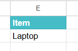
Step 2: Define criteria in a separate table. Here, the criteria tells Google Sheets to only consider rows where Item = Laptop.
Step 3: Click on any empty cell and type the following formula:
=DPRODUCT(A1:C7, “Cost”, E1:E2)

- A1:C7 → Database range (your inventory table).
- “Cost” → Field to use (this specifies the column values to multiply).
- E1:E2 → Criteria (in this case, only Laptop rows are selected).
Step 4: Press Enter
The function gives the total cost of laptops with ease.

You can expand the criteria table to include multiple rows (e.g., “Laptop” and “Smartphone”) and DPRODUCT will calculate the product for those items as well. This makes it very useful when analyzing specific categories of stock without manually filtering or writing separate formulas.
Example #3 – Calculate compound interest or investment growth by multiplying the principal, interest rate, and time fields for selected transactions
There is an investment firm that maintains a database of clients’ investments. Each record contains the fields like Client Name, Principal Amount, Annual Interest Rate, and Years Invested. We must calculate the growth value for a particular client using these fields. Instead of manual multiplication, we can use the DPRODUCT function to automate it.
Step 1: Create the database containing all the data with the criteria table.

Step 2: Let us now enter the following formula:
=DPRODUCT(A1:D6, “Rate”, F1:F2)
However, we want to multiply Principal × Rate × Time for the client ANC and Sons. To do that, we use DPRODUCT with the correct column references, as follows:
We apply DPRODUCT on each column and multiply results together:
=DPRODUCT(A1:D6, “Principal”, F1:F2) *
DPRODUCT(A1:D6, “Rate”, F1:F2) *
DPRODUCT(A1:D6, “Time (Years)”, F1:F2)

Step 3: Press Enter. For ABC and Sons:
- Principal = 50,000
- Rate = 6% (0.06)
- Time = 3 years
- → Growth Value = 50,000 × 0.06 × 3 = $9,000
So, the client’s investment growth over 3 years is $9,000.

While DPRODUCT itself doesn’t handle compounding directly, this approach helps quickly filter and compute investment growth for particular clients or specified conditions. DPRODUCT is handy when filtering through large client datasets.
Important Things to Note
- If the data is not structured, some alternatives to DPRODUCT include FILTER and PRODUCT, SUMPRODUCT and QUERY. However, these are more complicated to use compared to DPRODUCT.
- The cells featured in the criteria table should have the column header matching your table.
- DPRODUCT belongs to the category of database functions that work on structured data with criteria tables.
Frequently Asked Questions (FAQs)
We have the following uses:
The formula is used to calculate the total revenue for sales by multiplying the quantity by the cost per piece fields for particular products in a database.
It is used to compute the total value of inventory for inventory management by multiplying the quantity and the price for selected items.
It is used in financial modeling to calculate compound interest by multiplying the principal, interest rate, and time fields for selected transactions in a database.
Some of the functions similar to Google Sheets:
DPRODUCT – The formula is as follows: =DPRODUCT(A1:C6, “Price”, E1:E2). This multiplies the price values for rows matching the criteria.
DSUM – The formula for DSUM is: =DSUM(A1:C6, “Quantity”, E1:E2) – this function adds the quantity values for rows matching the criteria.
DAVERAGE – The formula is as follows: =DAVERAGE(A1:C6, “Cost”, E1:E2) – it is used to find the average cost for rows matching the criteria.
DPRODUCT can be used to filter data with conditions. Therefore, it only multiplies values for the records you want, unlike normal multiplication. Thus, it is useful when working with large databases where you only need results for specific entries. Alternatively, normal multiplication requires you to manually select and multiply each relevant value.
Use this DPRODUCT in Google Sheets Template to follow along with the examples in this article.
Download Excel Template