
What is CUMIPMT in Google Sheets?
CUMIPMT in Google Sheets stands for Cumulative Interest Payment. This function is used to calculate the total interest paid on a loan or investment between two specified payment periods. It helps us know how much of the payments we make go towards the interest over a specific time frame. This could range from a month to several years.
In a simple example, suppose a person takes a loan of $10,000 at an annual interest rate of 6% for 5 years. They must make monthly payments. To calculate the total interest paid in the first year, we use the following formula:
=CUMIPMT(6%/12, 5*12, 10000, 1, 12, 0)
In this formula, we enter the monthly interest rate, the total number of payments, and the loan amount. Periods 1 to 12 represent the first year, and 0 means payments are due at the end of the month. The result is the total interest paid during that period (it is a negative value since it’s an outgoing payment).

Use this CUMIPMT in Google Sheets Template to follow along with the examples in this article.
Download Excel TemplateKey Takeaways
- The CUMIPMT function in Google Sheets calculates the total interest paid on a loan over a specified range of payment periods.
- The syntax is as follows: =CUMIPMT(rate, nper, pv, start_period, end_period, type).
- CUMIPMT in Google Sheets focuses solely on the interest portion of loan payments, excluding any amount applied to the principal.
- It is useful for budgeting interest expenses, analyzing loan amortization, or evaluating interest-heavy phases of repayment.
- The function differs from CUMPRINC, which calculates the cumulative principal paid; CUMIPMT finds only the interest costs.
Syntax
The CUMIPMT in Google Sheets formula is as follows:
=CUMIPMT(rate, number_of_periods, present_value, start_period, end_period, end_or_beginning)
The arguments are as follows:
- rate – The interest rate per payment period.
- number_of_periods – The total number of payment periods.
- present_value – The principal or the present value of the loan or investment.
- start_period – The first period for which to calculate interest.
- end_period – The last period for which to calculate interest.
- end_or_beginning – Indicates whether payments are made at the end (0) or beginning (1) of each period.
How to Use CUMIPMT function in Google Sheets?
Did you know that the CUMIPMT function stands for Cumulative Interest Payment? As the name says, it calculates the total interest paid on a loan between two specific payment periods. This helps you figure out how much of your payments are going toward paying the interest, apart from reducing the loan balance.
We can enter CUMIPMT in two ways
- Use CUMIPMT by manually typing the formula
- By selecting it from the Google Sheets menu
Let’s first walk through the manual method using a simple example.
Entering CUMIPMT Manually
A person avails a $20,000 loan at a 5% annual interest rate. He must repay it monthly over 4 years. His bank manager wants to calculate the total interest paid in the first year (i.e., months 1 to 12).
Step 1:Enter the following loan details in a sheet, as shown below:

Step 2: In cell B8, we enter the following formula to find the interest payment over the first year. First, start by typing as shown below.
=CUMIPMT(

Step 3: Now, use the cell references for all arguments, in the order shown in the syntax.
=CUMIPMT(B1/12, B3*12, B2, B4, B5, B6)
This calculates:
- Monthly interest rate = B1/12
- Total number of payments = B3*12
- Present value = B2
- Start and end months = B4 to B5
- Type = 0 (for end of period)

Step 4: Press Enter. The result will show the total interest paid between months 1 and 12. You’ll see a negative value, as interest is an outgoing payment.

Step 5: To show the amount in dollars, just format the cell as $ by clicking on the symbol in the menu, as shown below.

Using CUMIPMT From the Google Sheets Menu
- Select the cell to display the value.
- Click on the Insert → Function → Financial.
- Choose CUMIPMT from the list of functions.
- Enter all the required arguments (either directly or using cell references).
- Press Enter to get the result.
Examples
Let us look at the examples below to understand how to use CUMIPMT in Google Sheets in different real-life scenarios.
It helps with budgeting, evaluating loan affordability, and analyzing interest-heavy early payments. Below are some CUMIPMT in Google Sheets examples showing how to apply CUMIPMT in everyday financial planning.
Example #1 – Calculate the Cumulative Interest Paid for a Loan Over a Specific Period
A person has taken a loan of $25,000 at an annual interest rate of 4.5%, to be repaid over 36 months with monthly payments. They want to calculate the total interest they will have paid in the first year of the loan.
(Before starting, always ensure the rate and number of periods are adjusted for the payment frequency.)
Step 1: Enter all the loan details as shown below:

Step 2: To calculate the total interest paid over the first 12 months, let us use the following formula in cell B8:
=CUMIPMT(B1/12, B3, B2, B4, B5, B6)

Step 3: Press Enter. The result will show the cumulative interest paid over the first year of the loan term.

Example #2 – Determine the Cumulative Interest Earned on An Investment Over a Given Duration
A career woman invests $15,000 in a fixed-income instrument that pays monthly interest at an annual rate of 6%. She invests it for a total duration of 5 years. She wants to calculate the total interest income she would earn over the first 18 months.
This function is useful in such scenarios for tracking short-term returns and understanding how much of the income is generated as interest during the investment period.
Step 1: Enter the required values into your Google Sheet: It is as shown below.

Step 2: Let us calculate the monthly interest rate. Also, verify the total number of payment periods:
- Monthly rate = 6% ÷ 12 = 0.5%
- Number of total periods = 5 years × 12 = 60
Step 3: To calculate cumulative interest for the first 18 months, enter the following formula in cell B8:
=CUMIPMT(B2/12, B4, B3, B5, B6, B7)

Step 4: Press Enter. We get the total interest earned from months 1 to 18. The result will be positive, indicating interest income received during this period of 18 months.

Using the CUMIPMT function not only helps you track your interest earnings accurately but also enables you to make smarter investment decisions.
Example #3 – Calculate the Cumulative Interest Accrued on Savings or Debts
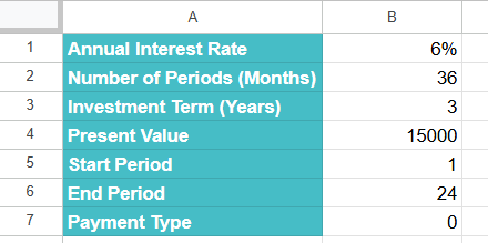
A lady opened a fixed deposit account with a bank and deposited $15,000 at an annual interest rate of 6%. The deposit is compounded monthly, and the term is 3 years. She wants to know how much total interest she will have earned by the end of the second year.
To calculate this, let us use the CUMIPMT in Google Sheets to determine the cumulative interest accrued over the first 24 months.
Step 1: Enter the following values in a given sheet:
Step 2: Enter the below formula in cell B7.
=CUMIPMT(B1/12, B2, B4, B5, B6, B7)
- B1/12: Monthly interest rate
- B2: Total periods (36 months)
- -B4: Present value (use negative sign for outflow/investment)
- B5: Start period (month 1)
- B6: End period (month 24)
- B7: Type (0 means payments at the end of period)

Step 3: Press Enter. The formula gives the total interest earned in the first two years of her investment. It appears as a positive value, since it’s an inflow or gain.

CUMIPMT in Google Sheets is a valuable tool for both savers and borrowers looking to understand the real impact of time and interest on their finances.
Important Things to Note
- Always check that the rate and number_of_periods are consistent with respect to their time units and not mixed. They should be in either months, quarters, or years.
- The start_period and end_period must be within the total number of payment periods to avoid errors.
- To calculate the monthly payments, divide the annual interest rate by 12. To get the total number of periods, multiply the number of years by 12.
- For quarterly payments, divide the annual interest rate by 4 and multiply the number of years by 4 for total periods. Similarly, for semi-annual payments, divide the annual interest rate by 2 and multiply the number of years by 2 for the total periods.
Frequently Asked Questions (FAQs)
The result of the CUMIPMT function in Google Sheets is a negative number because it represents the total interest paid, which is a cash outflow. Usually if it is a loan, the amount goes from the borrower to the lender, hence shown as a negative value. To make the outcome of the function as a positive number, you can wrap the formula with the ABS() function to remove the negative sign.
If the start_period or end_period in the CUMIPMT formula exceeds the total number of periods mentioned in the loan, the formula will return an error. The period range must be within the loan duration defined by the number_of_periods argument.
Some of the errors we get include:
The #NUM! Error occurs if
1. the given start_period or end_period is less than one
2. When either the rate, nper, or pv is less than or equal to zero.
3. The start period is greater than the end period.
The #VALUE! Error occurs if
1. Any of the argument values is non-numeric.
Use this CUMIPMT in Google Sheets Template to follow along with the examples in this article.
Download Excel Template