
What is INTRATE in Google Sheets?
The INTRATE function in Google Sheets calculates the interest rate for a fully invested security, such as a Treasury bill or a zero-coupon bond. This function assumes no periodic interest payments and is useful in financial analysis when determining the return on investment for short-term, discounted securities. It uses settlement and maturity dates, along with investment and redemption values, to calculate the implied annual interest rate.
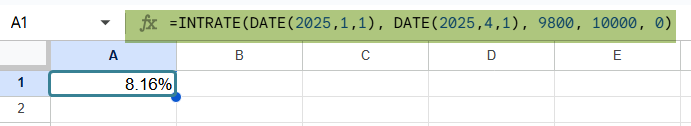
For example, if a company buys a bond for $9,800 that will pay $10,000 at maturity in 90 days, we use the below function to calculate the annual interest rate.
=INTRATE(DATE(2025,1,1), DATE(2025,4,1), 9800, 10000, 0)
This helps assess whether the return meets investment expectations or to compare it with other securities.
Use this INTRATE in Google Sheets Template to follow along with the examples in this article.
Download Excel TemplateKey Takeaways
- INTRATE calculates the interest rate for a discounted security like a Treasury bill, assuming simple interest over a single period.
- The syntax of the function is: =INTRATE(settlement, maturity, investment, redemption, [basis]).
- It is best suited for short-term, lump-sum investments where no intermediate payments are made.
- The function returns an annualized rate based on the time between settlement and maturity.
- Errors like #NUM! or #VALUE! can occur if dates are invalid or if the redemption is not greater than the investment.
Syntax
The syntax of the INTRATE function is as follows:
=INTRATE(settlement, maturity, investment, redemption, [basis])
Arguments:
- settlement: The date when the investment is purchased or settled.
- maturity: The date when the investment matures or is repaid.
- investment: The amount paid or invested initially.
- redemption: The amount received at maturity (the face value).
- basis (optional): The day count basis to use for the calculation. It can be:
- 0: US (NASD) 30/360 (default)
- 1: Actual/actual
- 2: Actual/360
- 3: Actual/365
- 4: European 30/360
This function returns the annual interest rate implied by the investment and redemption amounts over the time between the settlement and maturity dates.
How To Use INTRATE Function in Google Sheets
The INTRATE function is used to calculate the annual interest rate for an investment that does not pay periodic interest—like a Treasury bill or zero-coupon bond. It is useful in financial analysis when comparing returns on short-term securities or evaluating the profitability of cash-flow-free investments. This function can be used in two main ways:
- Entering the INTRATE function directly into a cell
- Using the Google Sheets menu
Entering INTRATE Directly
Let us look at an example. Suppose a company purchases a zero-coupon bond for $9,700 on April 1, 2025, which matures on October 1, 2025, and pays $10,000 at maturity. We want to calculate the implied annual interest rate.
Step 1: In your spreadsheet, enter the data as shown below.

Step 2: Click on an empty cell where you want the result. Type the function as follows:
=INTRATE(B1, B2, B3, B4)

We enter an = sign followed by the function name and the parameters separated by commas as stated in the syntax above.
Step 3: Press Enter. Format the result as a percentage. Google Sheets will return the annual interest rate based on the investment and redemption values over the specified period. You can use this result to compare it with interest rates from other investment options.

Using the Menu Bar
- Click the cell where you want the interest rate to appear.
- Go to the menu and navigate to Insert → Function → Financial → INTRATE.
- Once the function appears in the cell, enter the arguments in order: settlement date, maturity date, investment, redemption, and optionally, basis.
- Press Enter to calculate the result.
The cell now displays the computed interest rate, giving you a quick and clear financial insight.
Examples
The INTRATE function in Google Sheets calculates the annual interest rate for a fully invested, non-interest-paying security like a Treasury bill. Let us look at some practical examples to demonstrate the same.
Example #1 – Determine the Effective Interest Rate of An Investment
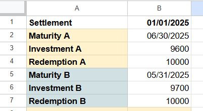
A startup is evaluating two short-term investment options for surplus funds that will not be used over the next few months. The company wants to compare the effective annual interest rate offered by these investments to make a data-driven decision.
To make a comparison, the team decides to use INTRATE in Google Sheets, which calculates the annualized rate of return for investments that don’t pay interest periodically like T-bills or short-term notes.
Step 1: Enter all the details in a sheet as shown below.
Step 2: In an empty cell, say B8, type:
=INTRATE(B1, B2, B3, B4)

This will return the annual interest rate for Investment A.
Step 3: In another empty cell B9, type:
=INTRATE(B1, B5, B6, B7)
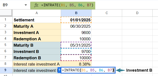
This will return the annualized rate for Investment B. Format both as percentages.
Step 4: Now compare the results in B8 and B9. The investment with the higher interest rate gives a better annual return, even if the maturity is shorter. This helps the company choose the more profitable option, accounting for both time and return.

By using the INTRATE function, businesses can accurately evaluate the true earning potential of short-term investments, helping them optimize their cash flow strategies without relying on guesswork.
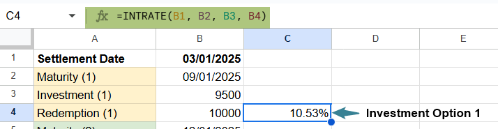
Example #2 – Analyze the Returns Generated by Different Investment Options
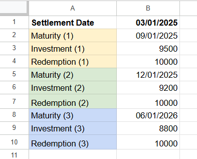
A financial analyst is comparing three investment products offered by different institutions. Each product has different investment amounts, maturity dates, and redemption values. To make an informed decision, the analyst wants to calculate the annual interest rate for each option using the INTRATE function in Google Sheets.
Step 1: Set up the investment data in a sheet, as shown below.
Step 2: Calculate the interest rate for Option 1.
In an empty cell, enter:
=INTRATE(B1, B2, B3, B4)
This gives the annual interest rate for Investment Option 1.
Step 3: Calculate the interest rate for Option 2
In another cell:
=INTRATE(B1, B5, B6, B7)
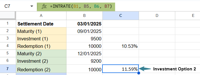
This calculates the return for Option 2.
Step 4: Calculate the interest rate for Option 3
=INTRATE(B1, B8, B9, B10)
This gives the annual rate for Option 3.
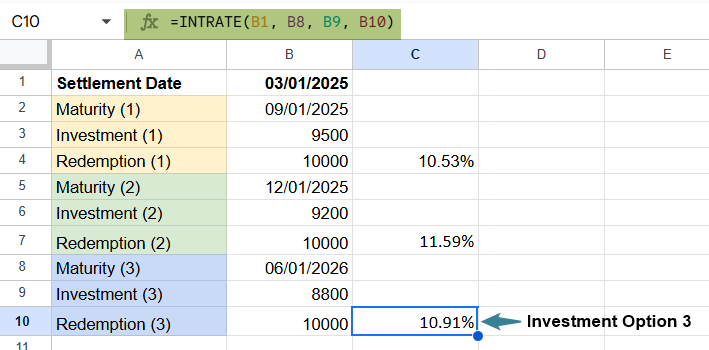
Review the interest rates calculated for each option to identify which investment provides the best return for the given time frame. This analysis helps prioritize short-term vs. long-term value.
Using INTRATE, we can make side-by-side comparisons of returns on various investments, giving a clear, consistent measure of performance—especially useful when maturity dates vary across products.
Example #3
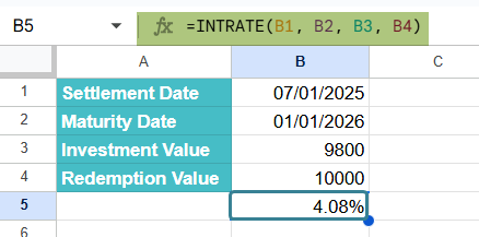
A small business decides to invest in a 6-month Treasury bill that pays a fixed amount at maturity. The company purchases the bill on July 1, 2025, for $9,800 and will receive $10,000 on January 1, 2026. The business owner wants to calculate the annual interest rate this investment will earn using the INTRATE function.
Step 1: Enter the investment data in a Google Sheet.
Click on an empty cell and type the following formula:
=INTRATE(B1, B2, B3, B4)

Press Enter.
Step 3: Check the result. Google Sheets returns the annual interest rate earned on this investment. This gives the business a clear picture of how much return it can expect on an annual basis.
This simple use of the INTRATE function is perfect for small businesses or individual investors who want to evaluate the return from short-term instruments like Treasury bills or promissory notes, where no periodic interest is paid.
Important Things to Note
- When using INTRATE in Google Sheets, both the settlement and maturity dates must be valid date values; otherwise, the function returns a #VALUE! error.
- The investment must be lower than the redemption (final amount), or the function will return a #NUM! error.
- The INTRATE function assumes a simple interest calculation over a single period (no compounding).
- By default, the day count basis is 0 (U.S. 30/360), unless specified.
- This function is ideal for instruments like Treasury bills, where interest is earned at maturity rather than through periodic payments.
Frequently Asked Questions (FAQs)
If the investment (initial) amount is higher than the redemption (final) value, the INTRATE function will return a #NUM! error. This is because the function assumes a gain from the investment, not a loss. The return rate cannot be negative in this function’s calculation.
The INTRATE function is best suited for short-term, single-period investments, like Treasury bills or simple promissory notes. It does not account for interest compounding or recurring coupon payments, which are common in long-term investments. For long-term investments with multiple payments, functions like YIELD or IRR would be more appropriate. Use INTRATE only when dealing with one-time maturity-based returns.
The optional basis parameter significantly affects the result, as it determines how days are counted in the year. For instance, U.S. (NASD) 30/360 assumes each month has 30 days, while actual/actual counts the real number of days. If we compare instruments across different regions or financial institutions, always confirm the day count method they follow. If omitted, the default basis is 0 (U.S. 30/360).
Use this INTRATE in Google Sheets Template to follow along with the examples in this article.
Download Excel Template