Highlight Every Other Row In Google Sheets

What Is Highlight Every Other Row In Google Sheets?

Highlight Every Other Row in Google Sheets helps users highlight or shade the alternate rows, even or odd, in a selected dataset. We can use desired unique colors, select from which row the colors must alternate, i.e., from row 1 or any other row.

The Google Sheets Highlight Every Other Row feature is useful when sorting data or while projecting reports to make it presentable that includes some features, such as Font/Text Style, Colour, Size, etc.

For example, in an empty worksheet let us select a cell range, here, A1:D7 and apply the Google Sheets Highlight Every Other Row feature, to get the following output.

We see that the alternate rows are of the same couple of colours, with the header highlighted in a darker shade.

How To Highlight Every Other Row In Google Sheets?

We can Highlight Every Other Row in Google Sheets in the following ways, namely:

1. Using Predefined Alternating Colors for alternate rows.
2. Using Custom Formula in Conditional Formatting.
3. Using Convert to Table Option for Alternate Colored Rows.

Method #1 – Using Predefined Alternating Colors for alternate rows

Step 1: Select the dataset or a cell range – select the “Format” tab – click the “Alternating colors” option, as shown below.

Step 2: The default alternating color appears for the selected cell range. The “Alternating colors” window appears on the right, where we can select the desired colors from the pre-defined “Default styles” section or customize using the “Custom styles” section and click “Done”, as shown below.

Method #2 – Uisng Formula in Conditional Formatting

Step 1: Select the dataset or a cell range – select the “Format” tab – click the “Conditional formatting” option, as shown below. Also, the “Conditional format rules” window appears on the right, there, click the “Add another rule” option.

Step 2: To add a rule, first, select the “Single color” tab and under the “Format rules” section, select the following:

• Click the “Custom formula is” option from the “Format cells if…” drop-down and type the formula “=MOD(ROW(),2)” in the value field that appears below.
• In the “Formatting styles” option, select the desired highlight color from the “Fill color”.
• Finally, click “Done”, as shown below.

[Special Note: The formula =Mod(Row(),2) works as follows:

1. The MOD function returns the remainder of the division calculation. For example, =MOD(3,2) returns 1. When we divide the number 3 by 2, we will get 1 as the remainder.
2. The ROW function returns the row number and the number returned will be taken as the first argument value by MOD and will be divided by 2.
3. If the remaining number returned by the MOD function equals number 1, Google Sheets will highlight the row by the mentioned color. If the row number is divisible by 2, the remainder will be zero and if the row number is not divisible by 2, we will get the remainder equal to 1.
4. Similarly, if we want to highlight every third row, we must change the formula to =MOD (ROW (), 3) =1.]

Method #3 – Uisng Convert to Table for Alternate Colored Rows

Step 1: Select the dataset or a cell range – select the “Format” tab – click the “Alternating colors” option, as shown below.

Step 2: The default alternating color appears for the selected cell range. The “Alternating colors” window appears on the right, where we can select the desired colors from the pre-defined “Default styles” section, here, orange, and click “Done”, as shown below.

Step 3: Now to convert to table option for alternate-colored rows, choose alternate rows coloured cell range A1:C5 – select the “Format” tab – click the “Convert to table” option, as shown below.

We get the following dataset and the “Alternating colors” window appears on the right, here as well, where we can select the desired colors from the pre-defined “Default styles” section or customize using the “Custom styles” section and click “Done”, as shown below.

Examples

We will consider some Highlight Every Other Row in Google Sheets examples to highlight alternate odd and even rows, and custom rows.

Example #1 – Highlight Every Other Row using the “Alternating colors” option

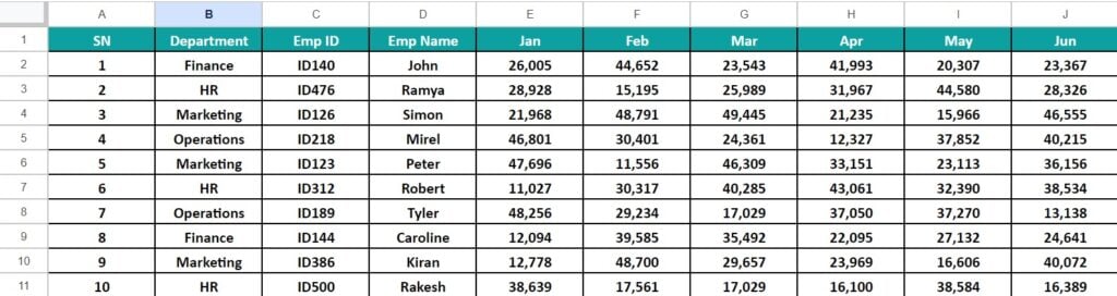
Consider the dataset that consists of the following employee details, such as the employee names, their IDs, departments and January to June salaries. We will Highlight Every Other Row in Google Sheets using the “Alternating colors” option.

The steps to highlight alternate rows are as follows:

Step 1: Select the cells A1:J11 – select the “Format” tab – click the “Alternating colors” option, as shown below.

Step 2: The default alternating color appears for the selected cell range. The “Alternating colors” window appears on the right, where we can select the desired colors from the pre-defined “Default styles” section, here, yellow, and click “Done”, as shown below.

Example #2 – Highlight Every Other Row with odd Number in Google Sheets

The dataset given below consists of grade 10 student details, such as their names, ID’s, Final scores and their promotion details. Let us Highlight Every Other ODD Rows using the Conditional formatting formula method.

The steps to highlight ODD alternate rows using the Conditional formatting method are,

Step 1: Select cells A1:F16 – select the “Format” tab – click the “Conditional formatting” option, as shown below. Also, the “Conditional format rules” window appears on the right, there, click the “Add another rule” option.

Step 2: To add a rule, first, select the “Single color” tab and under the “Format rules” section, select the following:

• Click the “Custom formula is” option from the “Format cells if…” drop-down and type the formula =ISODD(Row()) in the value field that appears below.
• In the “Formatting styles” option, select the desired highlight color, here “light orange” from the “Fill color”.
• Finally, click “Done”, as shown below.

The resulting dataset with ODD rows highlighted, is shown below.

Example #3 – Highlight Every Other Row with even number in Google Sheet

Consider the dataset of Example #2 once again. Let us Highlight Every Other Even Rows using the Conditional formatting formula method.

The steps to highlight EVEN alternate rows using the Conditional formatting method are,

Step 1: Select cells A1:F16 – select the “Format” tab – click the “Conditional formatting” option, as shown below. Also, the “Conditional format rules” window appears on the right, there, click the “Add another rule” option.

Step 2: To add a rule, first, select the “Single color” tab and under the “Format rules” section, select the following:

• Click the “Custom formula is” option from the “Format cells if…” drop-down and type the formula =ISEVEN(Row()) in the value field that appears below.
• In the “Formatting styles” option, select the desired highlight color, here “cyan” from the “Fill color”.
• Finally, click “Done”, as shown below.

The resulting dataset with EVEN rows highlighted, is shown below.

Important Things To Note

1. To take print outs, use light colors, because dark colors may not display the fonts clearly in the print-outs.
2. If the header is selected while applying conditional formatting, it will be treated as the first row.
3. We cannot change the color of the row once the conditional formatting is applied unless we update the format rule.
4. If we are unable to view the “Alternating colors” window, then use the path “Format 🡪 Alternating colors”.

Frequently Asked Questions (FAQs)

Download Template

This article must help understand Highlight Every Other Row In Google Sheets with its features and examples. You can download the template here to use it instantly.

Recommended Articles

Guide to What Is Highlight Every Other Row In Google Sheets. We learn to highlight alternate rows in different ways with step-wise examples. You can learn more from the following articles.-

Alphabetized In Google Sheets

Check Mark In Google Sheets

Absolute Reference In Google Sheets