
What is FVSCHEDULE in Google Sheets?
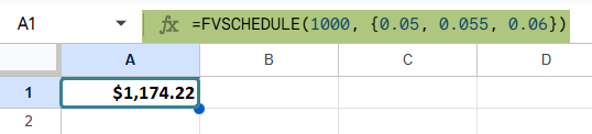
FVSCHEDULE in Google Sheets is a financial function that calculates the future value of an investment based on an initial principal and a series of interest rates. The usual basic compound interest formulas use a single rate, but FVSCHEDULE handles variable interest rates applied over multiple periods. This function is useful when the rate of return changes over time. This usually happens in the case of investments with fluctuating monthly, quarterly, or annual interest rates. Using FVSCHEDULE, one can see how their investment grows when each period has a different return rate. As an example, if you’ve invested $1,000 and the return rates over the next three years are 5%, 5.5%, and 6%. Here, there’s no fixed interest rate; hence, we use FVSCHEDULE to apply each rate sequentially to find the final value as follows.
=FVSCHEDULE(1000, {0.05, 0.055, 0.06})
This will calculate the future value of $1,000 after applying 5%, then 5.5%, then 6% interest, one after the other.
Use this FVSCHEDULE in Google Sheets Template to follow along with the examples in this article.
Download Excel TemplateKey Takeaways
- The FVSCHEDULE function calculates the future value of an investment by applying a sequence of interest rates, each compounded over time, making it ideal for modeling investments with fluctuating returns.
- The syntax of the function is as follows:
- =FVSCHEDULE(principal, schedule)
- It is commonly used in financial planning, investment forecasting, savings account modeling, or any scenario where interest rates vary across periods.
- All interest rates in the schedule must be numeric decimal values (not 6% but 0.06).
Syntax
The FVSCHEDULE in Google Sheets formula is as follows:
=FVSCHEDULE(principal, schedule)
- principal – The initial amount of money (investment).
- schedule – An array or range containing the series of interest rates to apply sequentially.
Each rate in the schedule is applied to the investment sequentially with compounding at each step.
How To Use FVSCHEDULE Function in Google Sheets?
The FVSCHEDULE function calculates the future value of an investment when interest rates change across different time periods. Instead of a single fixed rate, the function allows you to apply multiple interest rates at different schedules, compounded one after the other, sequentially. This function is useful when projecting investments like mutual funds or stock portfolios, with varying interest rates.
There are two ways to use this function in Google Sheets:
- By typing FVSCHEDULE directly into a cell
- Selecting it through the menu bar
Let’s go through the manual method first using a step-by-step example.
Manual Entry of FVSCHEDULE
A person has invested $1,500. He expects the returns over the next 4 years to be 5%, 6%, 4%, and 6.5% respectively. Let us use FVSCHEDULE to calculate the future value based on this rate schedule.
Step 1: In a column in Google Sheets, enter the required details, which are the interest rates(decimals).

Step 2: Enter the FVSCHEDULE formula as shown below. With an = sign, enter the formula name, open parentheses, followed by the arguments separated by commas.
=FVSCHEDULE(1500, A2:A5)
- 1500 is the principal amount (your original investment)
- A2:A5 contains the interest rate schedule (as decimals)

Step 3: Press Enter. The result shows the future value of their investment after compounding the interest rates in order.

Step 4: Here, the formula returns $1,849.13; it means that the $1,500 investment has grown to that amount after applying the three rates sequentially.
Using the Menu Bar
If you wish to enter through the menu, follow these steps:
- Select an empty cell.
- Go to Insert > Function > Financial > FVSCHEDULE
- Google Sheets will insert =FVSCHEDULE().
- Fill in the arguments manually.
- Press Enter to get the result.
Examples
To better understand how FVSCHEDULE in Google Sheets works in practical scenarios, let’s explore a few examples using some real-world data. These examples show how this function is especially useful for financial forecasting and growth tracking of portfolios.
Example #1
In this example, let us evaluate how an investment grows when interest rates vary over time. Such scenarios are common in personal finance and business planning. Here, the interest rates may change quarterly, annually, or according to the given market conditions.
The FVSCHEDULE function helps in calculating the future value of an investment based on a schedule of compound interest rates. We will use this function to determine how a principal amount grows when interest rates change over several periods. Here, the principal amount is $20,000. The rate of interest are given in Column A in a decimal form. Over four periods, the interest rates applied are 5%, 4%, 6%, and 3%, respectively.
Step 1: Enter the details as shown below.

Step 2: Enter FVSCHEDULE as shown below.
=FVSCHEDULE(B1, B2:B5)
- B1 is the initial investment amount.
- B2:B5 is the range of varying interest rates.

This function will return the future value of the investment after applying the listed rates sequentially.
Step 3: Press Enter. You get the future value of the investment after compounding the four interest rates in order. Use FVSCHEDULE to project investment growth realistically by applying different interest rates over time.

Example #2 – Using FVSCHEDULE with Named Ranges
In this example, let us calculate the future value of a seasonal investment using named ranges with the FVSCHEDULE function. Using named ranges makes the formula easier to read and more reusable—especially when interest rates change frequently.
A person runs a holiday store that opens seasonally. He invests $8,000 into the business at the start of each year. The returns vary based on the time of year, as holiday seasons yield better returns than off-seasons. We wish to find the future value at the end of the quarters.
Step 1: Enter the quarterly interest rates, as shown below.

Step 2: Create a named range by highlighting the cells B2:B5.
Go to Data -> Named ranges.

Name it (here we name it Returns) and click Done.
This will allow you to reference the rate schedule by name.

Step 3: Use FVSCHEDULE with the named range as shown below.
=FVSCHEDULE(8000, Returns)
This will apply each of the quarterly return rates to the $8,000 investment sequentially.

Step 4: Press Enter. The result is $9,223.03. That means your $8,000 investment grew to that amount after compounding across the four seasonal returns.

As we use a named range, we can also update the interest rates in cells A2:A5 and the formula automatically recalculates. This is a very useful feature when we use named ranges with FVSCHEDULE.
Example #3 – Using FVSCHEDULE with Negative Interest Rates
A woman runs an online business that keeps extra funds in a digital wallet that earns interest. There are some months when she gets positive interest from the platform, yet at other times, there may be negative interest or devaluation as well. She wants to track how her business reserves change over six months.
Her investment amount is $20,000, and the monthly returns are as shown below. We enter them in a sheet.
We’ll use FVSCHEDULE to calculate the actual future value of your reserves after six months of varying returns—including losses.
Step 1: Enter the monthly rates
In cells B1 to B6, enter the interest rates as decimals:

Step 2: Use the FVSCHEDULE function as shown below:
=FVSCHEDULE(20000, B1:B6)
Here:
- $20000 is your initial business reserve.
- A2:A7 contains monthly interest rates, including negatives.

Step 3: Press Enter. You’ll get the future value of your business reserve after 6 months.

The result $8,354.42 is the actual balance after compounding both positive and negative returns in order.
This formula allows you to model fluctuating returns with negative interest rates as well.
Important Things to Note
- FVSCHEDULE in Google Sheets requires the interest rates as decimal values, not percentages. For instance, 5% should be entered as 0.05. When you enter them as percentages, you will get incorrect answers.
- Interest rates in the schedule are applied sequentially, with each period compounding on the previous result. Hence, the order in which they are given matters.
- We can also include negative interest rates, which simulate losses or devaluation in a period.
- Named ranges work well with FVSCHEDULE, especially for scenarios where the interest rate list changes often.
- FVSCHEDULE works only with numeric inputs. If other types are entered, the function will return a #VALUE! error.
Frequently Asked Questions (FAQs)
If the range we enter in FVSCHEDULE includes a blank cell or non-numeric like text, the function will throw a #VALUE! Error. This is because the function expects every item to be a valid number in decimal form, and it sequentially multiplies them in a compound formula. A single blank can break the entire calculation. One can also wrap the range in a FILTER function to remove blanks or invalid values if necessary.
FVSCHEDULE is a flexible function that can be used for any time interval, be it monthly, quarterly, or annually. It depends on the interest rate schedule. However, the schedule must be consistent. All the interests given must reflect the same period. One should not mix a monthly rate with a yearly one for accurate results.
FVSCHEDULE handles negative and zero interest rates in its calculations. A negative rate reduces the investment’s value, simulating a loss. A zero rate keeps the value unchanged for that interval. Thus, FVSCHEDULE is extremely useful in real-world financial scenarios like recessions or idle account penalties.
Use this FVSCHEDULE in Google Sheets Template to follow along with the examples in this article.
Download Excel Template