
What is NOMINAL in Google Sheets?
NOMINAL in Google Sheets calculates the annual nominal interest rate given an effective annual interest rate and the number of compounding periods per year. It is used in financial calculations to convert an effective annual interest rate into a nominal annual rate. It finds the advertised rate before considering compounding. The NOMINAL function turns an effective annual interest rate into a nominal one. The effective rate is what one earns or pays in a year, including compounding. The nominal rate is the stated yearly rate without including compounding. Knowing the difference is easy to understand the real cost or return of a loan or investment.
For example, a person has an effective annual interest rate of 6.25%, compounded monthly. We can find the nominal rate as follows:
=NOMINAL(0.0625, 12)
The result is 6.08%, which is the nominal annual interest rate.

Use this NOMINAL in Google Sheets Template to follow along with the examples in this article.
Download Excel TemplateKey Takeaways
- NOMINAL calculates the nominal annual interest rate based on an effective rate and the compounding frequency.
- Its syntax is as follows: =NOMINAL(effect_rate, npery). There are two arguments: the effective annual rate (as a decimal) and the number of compounding periods per year.
- Understanding the difference between nominal and effective rates is critical for accurate financial analysis and decision-making.
- Using the NOMINAL function with other financial formulas like PMT increases the analytical knowledge for loans and investments.
Syntax
The NOMINAL interest rate formula in Google Sheets is straightforward:
=NOMINAL(effect_rate, npery)
The arguments stand for the following:
- effect_rate: This is the effective annual interest rate, which is the rate you earn or pay considering all compounding periods in a year.
- npery: It is the number of compounding periods per year. For instance, if your interest compounds quarterly, this would be 4.
How to Use NOMINAL Function in Google Sheets
The NOMINAL function is used to calculate the nominal annual interest rate given an effective interest rate and the number of compounding periods per year. It is useful in financial calculations regarding loans, investments, or savings accounts where interest is compounded more than once a year.
There are two ways to use NOMINAL in Google Sheets:
- Entering NOMINAL manually
- Selecting NOMINAL through the menu bar
Entering NOMINAL manually
Let’s walk through how to manually use the NOMINAL function:
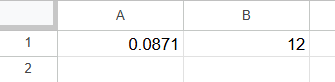
Step 1: Enter the data for the effective annual interest rate and the number of compounding periods. Here the data is as follows:
0.0871 (or 8.71%)
12 (for monthly compounding)
Step 2: Click on the cell where you want the nominal rate to appear and type the following function.
Enter the = sign and the function name.
Open the parentheses and enter the arguments in the order shown in the syntax, separated by commas.
Close the parentheses.
=NOMINAL(A1, B1)
One can also enter the numbers directly.
=NOMINAL(0.0871, 12)
This calculates the nominal interest rate based on 8.71% effective rate and 12 compounding periods.

Step 3: Press Enter. You get the nominal annual interest rate — in this case, around 0.084 or 8.4%.

TO make it a percentage value, click on the percentage symbol as shown below.

Using the Menu Bar
- Click the cell where you want the result to appear.
- Go to Insert > Function > All.
- Scroll through the list and click NOMINAL.
- Google Sheets will insert =NOMINAL() into the cell.
- Fill in the arguments and press Enter to get the result.
Examples
To understand the functioning of NOMINAL better, let us look at some real-life examples.
Example #1
A person wished to open a savings account and see one that advertises a 6.17% effective annual interest rate, compounded monthly. He wishes to know the nominal annual rate the bank is using to calculate monthly interest. This will help him understand how his money grows every month.
Let us use the NOMINAL function in Google Sheets to find out.
Step 1: Enter the data as shown below.
Enter the effective annual rate in decimal form (0.0617 for 6.17%).
Enter 12 as the number of compounding periods for monthly compounding.

Step 2: Apply the NOMINAL function as shown below.
=NOMINAL(B1, B2)
This calculates the nominal annual interest rate based on monthly compounding.

Step 3: You get the result after pressing Enter. Now to format as a percentage, click on cell B3. Go to Format -> Number -> Percent
It displays the result in percentage form.
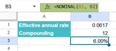
Thus, though the bank advertises an effective rate of 6.17%, the actual nominal rate being applied monthly is 6.00%. Hence, the bank is using a 6% annual rate and compounding it monthly — which grows to 6.17% over the year.
The difference clarifies how interest is applied monthly and helps make informed decisions when comparing accounts or planning investments.
Example #2 – Comparing Loan Options
In this example, let us evaluate two different loan offers with effective annual interest rates and varying compounding periods. Choosing the right loan requires not just comparing the effective rates, but also the nominal interest rates to make an accurate comparison.
This method is commonly used in personal finance, banking, and investment analysis to assess which loan or investment product offers the best value over time. Here, let us look at how the borrower compares the two loans.
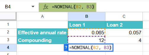
Step 1: Enter all the details regarding the loans in a Google Sheet.
One must decide between two loan offers:
Loan 1: 6.5% effective annual rate, compounded monthly (12 periods).
Loan 2: 5.7% effective annual rate, compounded quarterly (4 periods).
You want to determine which loan has the lower nominal annual rate, making it more cost-effective.

Step 2: Apply the NOMINAL function as shown below in cell B4.
=NOMINAL(B2, B3)
This calculates the nominal annual rate based on the corresponding effective rate and compounding frequency.
Step 3: Press Enter and drag the formula to cell C4.
Now compare both the rates. We see that that Loan 2 has a lower effective annual rate, the nominal rate also turns out to be slightly lower than Loan 1. This confirms that Loan 2 is the better financial choice, assuming all other terms are equal.

Example #3
An analyst is evaluating a savings account with a 6.2% effective annual rate. It is compounded monthly, for a $10,000 deposit. The bank offers a bonus interest if the nominal annual rate is more than 6%. He wished to calculate the nominal annual rate using NOMINAL and determine if the person is eligible for the bonus using IF.
Step 1: Enter all the details in a Google Sheet.

Step 2: Calculate the Nominal annual rate as shown below in an empty cell.
We use the following formula with IF function to check if they are eligible for a bonus.
=IF(NOMINAL(B1, B2) > 6, “Eligible”, “Not eligible”)

Step 3: Press Enter. You can find if the account is eligible for a bonus.

Using the NOMINAL and IF combination, we can evaluate if the person qualifies for a bank’s bonus interest offer. In this case, they are not eligible.
Important Things to Note
- Ensure that the effective interest rate provided as the argument aligns with the compounding periods per year. If the effective rate is annual, npery should be 1.
- Compounding frequencies can be annual, semi-annual, quarterly, monthly, or any other period, and the value of npery should reflect this accurately.
- The nominal interest rates do not account for the effects of compounding. They represent the annual interest rate without considering compounding periods.
- Format the cell or the formula output to display the results as percentages or in other desired formats, depending on your requirements.
Frequently Asked Questions (FAQs)
Some of the errors you get when using the NOMINAL function include:
If the arguments effect_rate, npery are nonnumeric, the function returns the #VALUE! error value. If either the effect_rate ≤ 0 or if npery < 1, NOMINAL returns the #NUM! error.
Some financial functions similar to NOMINAL function include:
EFFECT(rate, npery) – This function alculates the effective annual interest rate from a nominal rate and number of compounding periods.
FV(rate, nper, pmt, [pv], [end_or_begin]) – the FV function finds the future value of an investment or loan based on periodic payments and a constant interest rate.
PV(rate, nper, pmt, [fv], [end_or_begin]) – This function returns the present value of a series of future payments. Can be used for investment analysis.
Some of the common errors to look for when using the NOMINAL function:
1. Enter the correct nominal effective rate: Always ensure the effective rate is in decimal form as entering it as a whole number will lead to incorrect results.
2. Always check the number of compounding periods.
3. Google Sheets returns a decimal by default. Format the cell as percentage to view it as a percentage like 6.17%.
Use this NOMINAL in Google Sheets Template to follow along with the examples in this article.
Download Excel TemplateRecommended Articles
Continue with these related resources when you want the next practical step in this topic.
- PV in Google Sheets
- FV in Google Sheets
- NPV in Google Sheets
- IRR Google Sheets Function
- PMT in Google Sheets
Explore the full Google Sheets Financial Functions guide or browse Google Sheets Resources.