What Is Compound Interest In Excel Formula?
The Compound Interest formula in Excel gives the interest amount on savings estimated on the initial principal and accumulated interest from the previous periods.
Users can use the Excel Compound Interest formula to evaluate the compound interest non-annually, and the appreciation and depreciation in commodity prices. And it also helps determine the inflation in profit and loss.
For example, the table below contains the inputs required for the monthly compound interest calculation.
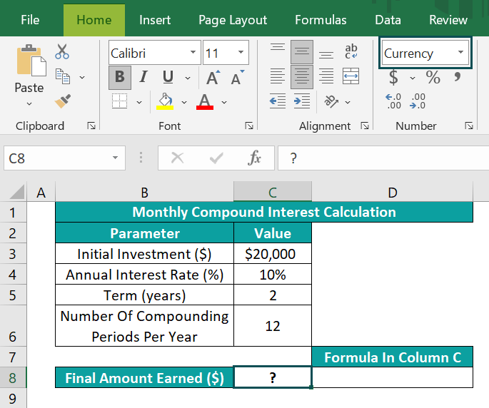
If the data format in the target cell C8 is set as Currency, then, we can apply the monthly Compound Interest formula in Excel cell C8, and achieve the final amount earned.
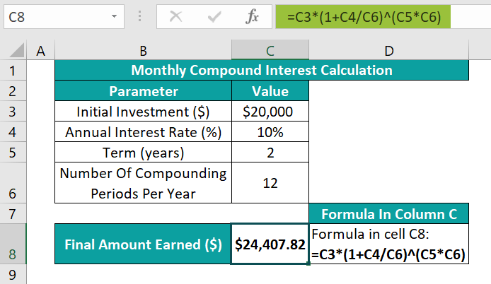
The compounding frequency each year is 12. And the formula divides the yearly interest rate by 12 and multiplies the Term by 12, as the interest gets compounded every month in a year.
📥Download the ready-to-use Excel template to practice this tutorial yourself.
Compound Interest Formula In ExcelAnd the result in cell C8 is the overall accumulated sum, which includes the initial investment and the compound interest.
Thus, based on the above monthly Compound Interest formula calculation, the interest earned in the first month will be $20,000*(10%/12), which is $166.66. And in the second month, it will be ($20,000+$166.66)*(10%/12), which is $168.055, and so on every month for two years, arriving at a total of $24,407.82.
Table of contents
Key Takeaways
- The Compound Interest formula in Excel determines the interest on the initial investment and the interest accrued over the previous periods.
- The compounding frequency each year for the interest compounded semi-annually, quarterly, monthly, and daily is 2, 4, 12, and 365, respectively.
- Users can use the compound interest expression to evaluate the returns earned on the money they invested initially and after each compounding period.
- We can apply the compound interest expression in a worksheet using the mathematical expression, the calculation table, and Excel inbuilt functions FVSCHEDULE and FV.
How To Calculate Compound Interest In Excel Formula?
We can Calculate Compound Interest In Excel Formula in the following ways, namely,
- Using Mathematical Compound Interest Excel Formula.
- Using the Compound Interest Calculation Table in Excel.
- Compound Interest Using FVSCHEDULE Excel Formula.
- Compound Interest Using the FV Excel Formula.
We will consider specific examples for each of the above-mentioned ways to determine compound interest in Excel.
Example #1 – Using Mathematical Compound Interest Excel Formula
The mathematical expression to determine the compound interest is as follows:

where,
- P: The principal amount or the initial investment
- r: The yearly interest rate
- n: The compounding frequency each year
- t: The total period for which one applies the interest.
And the Total Accumulated Amount includes the initial investment and the compound interest.
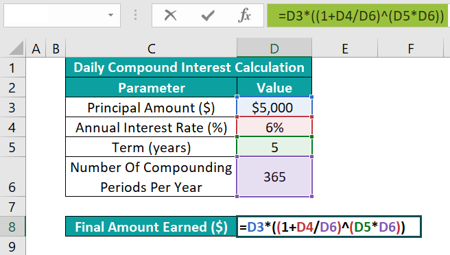
For example, the table below contains the inputs required for the daily compound interest calculation.

The steps to apply the daily Compound Interest formula in Excel cell D8 and achieve the final amount earned are,
- Step 1: Select cell D8, and enter the formula =D3*((1+D4/D6)^(D5*D6)).
- Step 2: Press Enter to view the final accumulated sum.
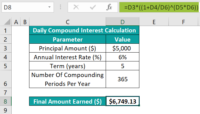
The compounding frequency each year is 365. And the formula divides the yearly interest rate by 365 and multiplies the Term by 365, as the interest gets compounded daily or 365 times per year.
And the result in cell D8 is the overall accrued sum, which includes the principal and the compound interest.
Thus, based on the above daily Compound Interest formula calculation, the interest earned on the first day will be $5,000*(6%/365), which is $0.82. And on the second day, it will be ($5,000+$0.82)*(6%/365), which is $0.82205, and so on every day for five years, making a total of $6,749.13.
Furthermore, the following table shows the standard compounding frequency per year data used in the compound interest calculations and their interpretation.

We can refer to the above table when evaluating the non-annual compound interest values.
Example #2 – Using Compound Interest Calculation Table in Excel
Using a calculation table, we shall see how to apply the quarterly Compound Interest formula in Excel.
For example, the table below shows the initial investment in period 0 and the yearly interest rate in cells E3 and H2, respectively. We will determine the amount earned at each quarter end and display the output in cells E4:E7.
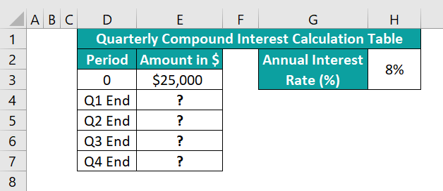
The steps to apply the quarterly Compound Interest formula in Excel using a calculation table are,
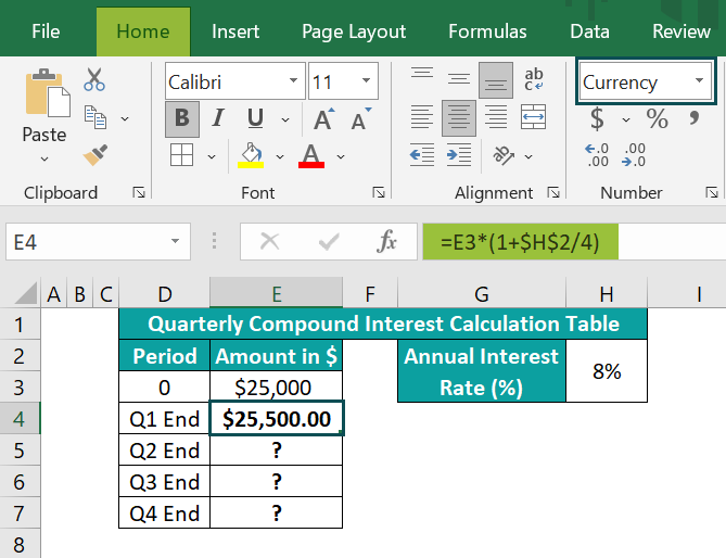
- Step 1: Select the target cell E4, enter the formula =E3*(1+$H$2/4), and press Enter.
- Step 2: Using the fill handle in excel, implement the formula in the remaining target cells E5:E7.
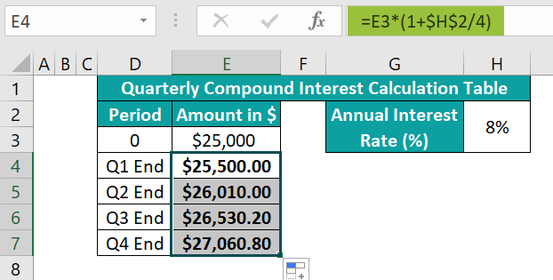
The formulas in cells E4: E7 return the investment’s future value after each quarter, from Q1 to Q4. And we divide the yearly interest rate by 4 in the above formula as we require the interest, compounded quarterly.
Furthermore, the total amount earned at the fourth quarter end is $27,060.80, which includes the principal sum and the compound interest.
Example #3 – Compound Interest Using FVSCHEDULE Excel Formula
We shall see the method to execute the half yearly Compound Interest formula in Excel using the inbuilt FVSCHEDULE function.
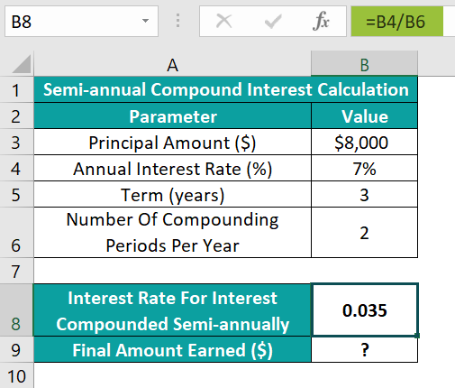
For example, the table below shows the inputs required to achieve the interest compounded semi-annual in cell B9.
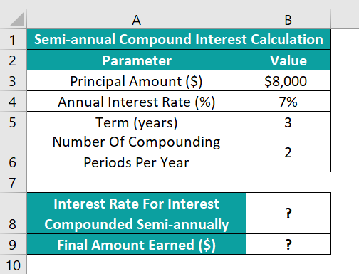
The steps to implement the half yearly Compound Interest formula in Excel using the inbuilt function FVSCHEDULE in the target cell.
- Step 1: Select cell B8, enter the formula=B4/B6 to determine the interest rate for the interest compounded semi-annually, and press Enter.
- Step 2: Select cell B9, enter the formula =FVSCHEDULE(B3,{0.035,0.035,0.035,0.035,0.035,0.035}), and press Enter.
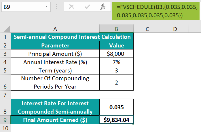
The FVSCHEDULE() accepts,
- the principal sum of $8,000 as the first argument, principal, which is the present value.
- And its second argument is the schedule, which is the array of interest rates we must apply.
In the above example, as the compounding frequency in each year is 2, and the total terms are 3, the array range must include 6 interest values. And the interest rate to use is 0.035, which we calculated in cell B8.
Thus, based on the input argument values, the FVSCHEDULE() returns the accrued amount as $9834.04. And it is the initial investment’s future value, with a series of compound interests.
Example #4 – Compound Interest Using the FV Excel Formula
Let us see how to determine the quarterly compound interest using the FV function in excel.
The table below contains the inputs required to obtain the interest compounded quarterly.
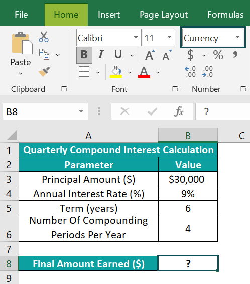
The steps to use the FV() in the target cell to determine the accumulated sum at the sixth year’s last quarter end are as follows:
- Step 1: Select the target cell B8, enter the FV() formula =FV(B4/B6,B5*B6,0,-B3), and press Enter.
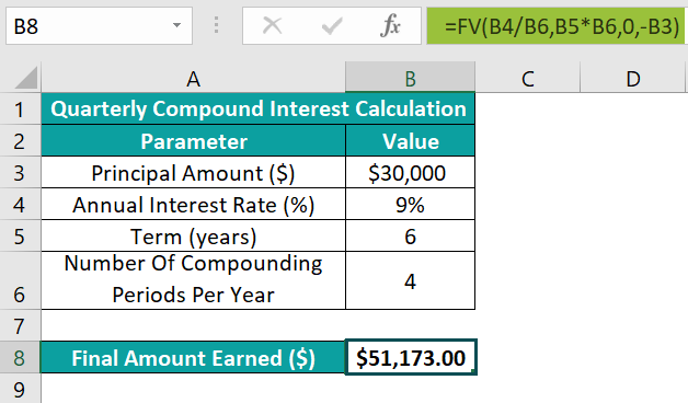
[Special Note: The FV() arguments are rate, nper, pmt, pv, and type.
- The rate argument indicates the interest rate per period in a series of regular payments. So, we pass the argument value as the yearly interest rate divided by compounding frequency per year. And the argument nper is the total number of periods of regular payments, which is the product of the Term and compounding frequency per year.
- On the other hand, we must supply pmt or pv. And as we do not add any additional cost to the initial investment in the investment period, we will set the pmt argument value, which is the payment in each period, as 0.
- So, as we ignore the argument pmt, we must provide the argument pv value, which is the present value or the principal sum. And as theamount is an investment, it will be a negative value.
- And the last argument, type, is optional, which we shall ignore, as the example considers the payment is due at every period end.]
Thus, based on the supplied input values, the FV() returns the accumulated sum at the sixth year’s end, $51,173. And it is an amount that includes the initial investment and the compound interest.
Important Things To Note
- The input values used in the Compound Interest formula in Excel must be of the correct data types.
- We will get the #VALUE! Error if the FVSCHEDULE and FV functions’ argument values are non-numeric.
- Ensure the supplied present value to the FV() is negative, as it is an outgoing amount.

Frequently Asked Questions (FAQs)
Excel can calculate compound interest. The following methods help us achieve the increased amount, which includes the initial investment and the compound interest.
• Using mathematical compound interest expression
• Using the compound interest calculation table
• Using the FVSCHEDULE function
• Using the FV()
The difference between simple interest and Compound Interest formula in Excel is that the simple interest formula calculates the interest on the principal amount of a loan. On the other hand, the compound interest expression determines the interest on the principal amount and the accrued interest in the previous periods.
For example, the tables below contain the inputs required to determine the simple and semi-annual compound interests in cells B8 and E8.
The steps to perform the required calculations are,
• Step 1: Select the target cell B8, enter the simple interest formula =B3*B4*B5, and press Enter.
The formula multiplies the principal, yearly interest rate, and the time to return the simple interest accrued when the loan period ends.
• Step 2: Select the target cell E8, enter the formula=E3*((1+E4/E6)^(E5*E6)), and press Enter.
The above formula returns the initial investment’s future value plus the compound interest.
The Compound Interest formula in Excel might not work for the following reasons:
• The input values supplied to the compound interest expression are of the incorrect data types.
• The compounding frequency per year does not match the non-annual compound interest calculation requirement.
• The supplied arguments to the FVSCHEDULE() or FV() are non-numeric or blank cells.
• The initial investment supplied as the pv argument value to the FV() is not negative.
Download Template
📥Download the ready-to-use Excel template to practice this tutorial yourself.
Compound Interest Formula In ExcelRecommended Articles
This has been a guide to Compound Interest Formula In Excel. Here we explain the top 4 method to calculate it along with examples & downloadable template. You can learn more from the following articles –

Leave a Reply