
What Is FV Excel Function?
The FV in Excel stands for the Future Value and is categorized under Financial functions. In simple words, the Future Value function calculates the future value of investments. It is calculated on the discount rate, number of periods of investments, and present value of the payment.
FV is used in financial projects. For instance, FV evaluates low-risk investments, the interest paid on loans, and many more. For example, assume ABC Bank’s bond has invested $10,000. Also, the interest rate is 10% for ten years. Now, we need to calculate FV in Excel using the below steps.

The steps used to calculate FV in Excel are as follows:
Use this FV in Excel Template to follow along with the examples in this article.
Download Excel TemplateStep 1: First, select an empty cell to display the output.
In this example, let us select cell B5.
Step 2: Next, enter the FV formula in cell B5 to calculate the Future Value of the Investment.
The entered formula is =FV(B2,B4,B3,0,0)
Step 3: Then, press Enter key.
Clearly, we can see that the function has returned the output in cell B5.

Likewise, we can calculate FV in Excel for the given data.
Formula of Future Value
The formula of FV is:
FV = PV * (1+r)ᵑ
where,
- FV = Future Value
- PV = Present Value
- r = Rate of Interest
- n = the number of years
Key Takeaways
- The formula of Future Value is FV = PV * (1+r)ᵑ and,
- FV = Future Value
- PV = Present Value
- r = Rate of Interest
- n = the number of years
- The FV calculates the Future Value of investments, loans, etc. Generally, the fixed payment needs to be done at every set time.
- The payment amount of cash outflow should be negative (e.g., $-1000), and the payment amount of cash inflow should be positive (e.g., $1000).
- The Future Value function is used in financial calculations.
FV Excel Formula
The syntax of the FV Excel Function is
where,
- rate: It is a mandatory argument and it refers to the rate of interest or discount rate.
- nper: It is a mandatory argument and it denotes the number of periods of annuity or investment.
- pmt: It is a mandatory argument and it shows the payment made per period with principal amount and interest.
- pv: It is an optional argument representing the present value of investment or loans.
- type: It is also an optional argument, showing whether the payment is made at the starting or end of the period.
The value is 0 or 1; 0 is for payment made at the end, and 1 is for payment made at the beginning.
How To Calculate Future Value In Excel? (With Steps)
We can use the following 2 methods to obtain output using FV in Excel:
1. Access From The Excel Ribbon
- First, go to the Formulas tab.
- Next, click on the Financial option from the Function Library group.
- Then, click on the FV function from the drop-down list.
- The Function Arguments window pops up.
- Then, enter the arguments in the Rate, Nper, Pmt, Pv & Type
- Click OK.
2. Enter The Worksheet Manually
- First, select an empty cell to display the output.
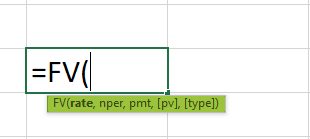
- Type =FV( in the selected cell. Alternatively, type =F and double-click the FV function from the list of suggestions shown by Excel.
- Then, enter the arguments as excel cell references or direct values.
- Close the parenthesis and press the Enter key.
Let us look at a basic example of FV formula in excel –
Mr. Peter has invested $5000 in a company’s bond. The interest rate for five years is 5%. Now, let us learn how to find FV in Excel using the following steps.
In the table,
- Column A shows the investments.
- Column B highlights the data.

The steps to obtain output using FV in Excel are as follows:
Step 1: To begin with, select an empty cell to display the output.
So, we have selected cell B5 in this example.
Step 2: Next, start by entering the formula in cell B5.
Step 3: Then, select the cell that contains the rate, i.e., B2.

Step 4: Now, choose the cell that contains the number of periods, i.e., B4.

Step 5: Also, select the cell that contains the investment per period, i.e., B3.

Step 6: Then, enter the present value, i.e., 0.

Step 7: Finally, we should also enter the period type, i.e., 0-end of the period.

So, the complete formula is =FV(B2,B4,B3,0,0).
Step 8: Press Enter key.
We will obtain the result in cell B5, as shown in the below image.

Similarly, we can find the output using FV in Excel.
Examples
Example – 1 – Calculating FV When PV Amount Is Given
The Present Value is $2,000 and the interest rate is 10%. The period of installments is also 10. So, we need to use the below steps to understand how to find FV in Excel.
In the table,
- Column A shows the investments
- Column B displays the data

The steps used to find FV in Excel are as follows:
Step 1: To begin with, select an empty cell to display the output.
We have selected cell B5 in this example.

Step 2: Next, start by entering the formula in cell B5.
Step 3: Then, select the cell that contains the rate, i.e., B2.
Step 4: Also, choose the cell that contains the number of periods, i.e., B4 for the next argument.
Step 5: If the investment amount is not given, the space is left in the formula.
Step 6: Next, select the cell that contains the Present Value, i.e., B3.
Step 7: Then, enter the period type, i.e., 0-end of the period.
So, the complete formula is =FV(B2,B4, ,B3,0).
Step 8: Press Enter key.
We will get the output in cell B5, as shown in the image below.

Therefore, we can find the output using FV in Excel.
Example – 2 – Calculating FV With Monthly And Quarterly Installments.
Calculating FV With Monthly Installments
The below table shows investments and data in columns, A and B. The monthly installment is $100, the interest rate is 10%, the number of years is 5, and the payment per year is 12. Therefore, we need to use the below steps to calculate FV in excel with monthly installments.

The steps used to find FV in Excel are as follows:
Step 1: To begin with, select an empty cell to display the output.
We have selected cell B6 in this case.

Step 2: Next, start by entering the formula in cell B6.
Step 3: Then, select the cell that contains the rate according to the month, i.e., B2/B4.
Step 4: Now, select the cell that contains the number of years and monthly installments, i.e., B5*B4.
Step 5: Also, select the cell that contains the Investment per period, i.e., B3.
So, the complete formula is =FV(B2/B4,B5*B4,B3).
Step 6: Press Enter key.
We will get the FV output in cell B6 as shown in the image below:

Thus, we can calculate FV in Excel with ease.
Calculating FV With Quarterly Installments
The quarterly installment is $500, the interest rate is 10%, the number of years is 5, and the payment per year is 4. But, first, let us understand how to find FV in Excel when a quarterly installment is given.
In the table,
- Column A shows the investments.
- Column B displays the data.

The steps used to find FV in Excel are as follows:
Step 1: To begin with, select an empty cell to display the output. We have selected cell B6 in this case.
Step 2: Next, start by entering the formula in cell B14.
Step 3: Then, choose the cell that contains the rate according to the quarter, i.e., B10/B12.
Step 4: Next, select the cell that contains the number of years and quarterly installments, i.e., B13*B12.
Step 5: Finally, select the cell that contains the Investment per period, i.e., B11.
So, the complete formula is =FV(B10/B12,B13*B12,B11).
Step 6: Press Enter key.
Excel returns the output in cell B6, as shown in the image below.

Likewise, we can find FV in Excel.
Example – 3 – Calculating FV To Compare Two Investments
Mr. Sam has invested money in two projects. For $1000 in Project A, the interest rate is 10%, and the duration is five years; for $2000 in Project B, the interest rate is 10%, and the time is five years. Let us understand how to find FV in Excel and compare these two investments using FV in Excel.
Project A:
The investment value is $1000, the interest rate is 10%, and the number period is five years.
The table shows the investment done by Mr. Sam in Project A; we need to find FV in Excel.
In the table,
- Column A shows the investments.
- Column B displays the data.

The steps to calculate FV are as follows:
Step 1: To begin with, select an empty cell to display the output. We have selected cell B6 in this case.
Step 2: Next, start by entering the formula in cell B6.
Step 3: Then, choose the cell that contains the rate, i.e., B3.
Step 4: Also, select the cell that contains the number of periods, i.e., B5.
Step 5: Next, select the cell that contains the Investment per period, i.e., B4.
Step 6: The present value and the period type arguments are optional. If we do not enter, excel automatically treats it as 0.
So, the complete formula is =FV(B3,B5,B4).
Step 7: Press Enter key.
We get the results as shown in the image below.

Project B:
The investment value is $2000, the interest rate is 10%, and the number of the period is five years.
In this example, the table shows the investment done by Mr. Sam in Project B; we need to find FV in excel.
In the table,
- Column A shows the investments.
- Column B displays the data.

The steps used to find FV in Excel are as follows:
Step 1: First, select an empty cell to display the output. We have selected cell B13 in this case.

Step 2: Next, start by entering the formula in cell B13.
Step 3: Then, select the cell that contains the rate, i.e., B10.
Step 4: Now, select the cell that contains the number of periods, i.e., B12.
Step 5: Next, select the cell that contains the Investment per period, i.e., B11.
Step 6: The present value and the period type arguments are optional, and if we do not enter, the formula automatically treats the value of PV as 0.
So, the complete formula is =FV(B10,B12,B11).
Step 7: Press Enter key.
Excel returns the output in cell B6, as shown in the image below.

Though the investment made in both the projects differ, all other arguments remain the same.
So, the calculated Future Value differs.
Important Things To Note
- The #VALUE! error occurs when non-numeric arguments (such as text and symbols) are passed.
- The ‘0’ is given to the ‘type’ argument when the payment of investments is made at the end of the month.
- The PV argument is optional but becomes mandatory if compound interest is calculated.
- The Nper and rate values must be consistent for all the months.
- The FV in Excel function is an easy method used to calculate investments.
- The rate can be in percentage or decimal form.
Frequently Asked Questions (FAQs)
FV stands for Future Value, which calculates the future value of investments or loans made.
The formula of the FV function in Excel is =FV(rate,nper,pmt,[pv],[type])
For example, consider the below table where investment payment is $8,000 with a 2% interest rate. Also, the payments are made monthly, and we will do so for five years. Let us learn how to find FV in Excel with the below steps.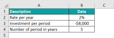
The steps used to find FV in Excel are as follows:
Step 1: To begin with, choose the cell to enter the FV formula.
In this case, let us select cell B5.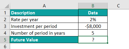
Step 2: Next, enter the FV formula in cell B5 to calculate the Future Value of Investment.
The entered formula is =FV(B2/12,B4*12,B3,0,0).
Here, the interest rate is divided by 12, and the period is multiplied by 12 because the investment is made every month. We need to calculate the Future Value according to the year.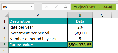
Likewise, we can calculate FV in excel with ease.
We can insert the FV function using the below steps:
1. First, we should select the cell.
2. Then, type the formula =FV(….
3. Next, select the rate, nper, pmt, pv, and type.
4. Press Enter.
We can obtain results using FV in Excel either manually or by using the below steps:
1. To begin with, select the cell which has the number.
2. Next, go to the Formulas tab.
3. Click on the Financial option and select the FV option from the drop-down list.
4. The Function Arguments window pops up.
5. Then, enter the value in the Rate, Nper, Pmt, Pv, and Type as the number of arguments.
6. Click OK.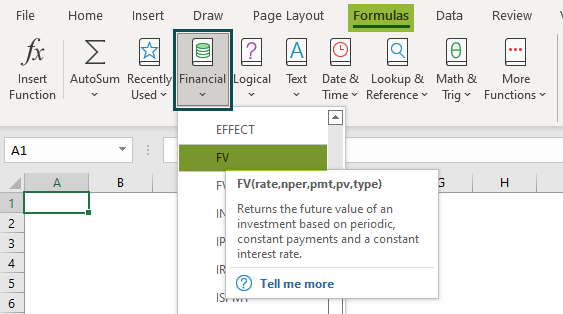
Use this FV in Excel Template to follow along with the examples in this article.
Download Excel TemplateRecommended Articles
Continue with these related resources when you want the next practical step in this topic.
Explore the full Excel Financial Functions guide or browse Excel Resources.