
What Is COUNTUNIQUE In Google Sheets?
The COUNTUNIQUE in Google Sheets checks and detects the unique values in a selected dataset or a cell range and returns the count of the values.
The Google Sheets COUNTUNIQUE function helps users to identify the unique values, not taking into count their duplicates or repeats, and gets the precise count while generating reports.
Use this COUNTUNIQUE In Google Sheets Template to follow along with the examples in this article.
Download Excel TemplateFor instance, we have some random repeated or duplicated data. We will use the COUNTUNIQUE() formula to get the count of only the unique items excluding the duplicate ones.
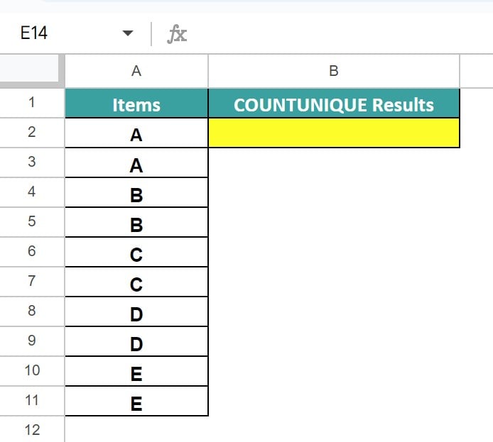
Select cell B2, enter the formula =COUNTUNIQUE(A2:A11) and press “Enter”, as shown below.

The output is 5, because there are 5 alphabets that are repeated.
Key Takeaways
- COUNTUNIQUE in Google Sheets is a Math function available in Google Sheets and not in MS Excel. It searches and counts the data only once, ignores its duplicates and returns the count.
- It is case sensitive, which means if the values are A and a, they are considered as 2 different values and not repeated or duplicate.
- The dataset retrieved will be without formatting. We can format it as required once we get the final data to comprehend clearly.
- We can use the COUNTUNIQUEIFS to count unique values with single or multiple criteria.
- We must remember that we cannot insert the COUNTUNIQUEIFS function as we insert the COUNTUNIQUE, because the COUNTUNIQUE is under the MATH category and the COUNTUNIQUEIFS falls in the Statistical category. However, we can us the ALL category to insert any of the COUNT family functions as shown in FAQ1.
Syntax
The syntax of the COUNTUNIQUE Google Sheets Formula is,

The arguments of the COUNTUNIQUE Google Sheets Formula are,
- value1 – It is the cell range or the dataset to check and count the unique values. It is a mandatory argument.
- [value2, value 3, …] – It is an optional argument used when we have to select multiple cell ranges.
How To Use COUNTUUNIQUE In Google Sheets?
We can use the COUNTUNIQUE In Google Sheets in 2 ways, namely,
- Access from the Google Sheets ribbon.
- Enter in the worksheet manually.
Method #1 – Access from the Google Sheets ribbon –
Step 1: Choose an empty cell for the output – select the “Insert” tab – click the “Function” option right arrow – click the “Math” option right arrow – select the “COUNTUNIQUE” function, as shown below.

Step 2: The “COUNTUNIQUE” formulaappears, as shown below. Enter the argument as cell reference.

Method #2 – Enter in th worksheet manually –
Step 1: Select an empty cell for the output.
Step 2: Type = COUNTUNIQUE ( in the cell. [Alternatively, type =C or =COUNT and double-click the COUNTUNIQUE function from the Google Sheets suggestions.]
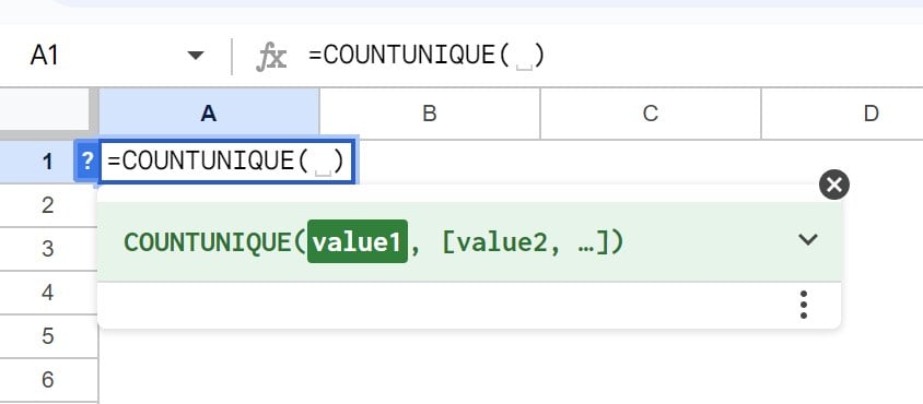
Step 3: Enter the arguments as cell values or cell references and close the brackets.
Step 4: Press Enter to view the outcome.
Examples
Let us consider specific COUNTUNIQUE in Google Sheets examples and count unique cells using the COUNTUNIQUEIFS(), IF() and DATE() functions.
Example #1 – Use COUNTUNIQUE function In Google Sheets.
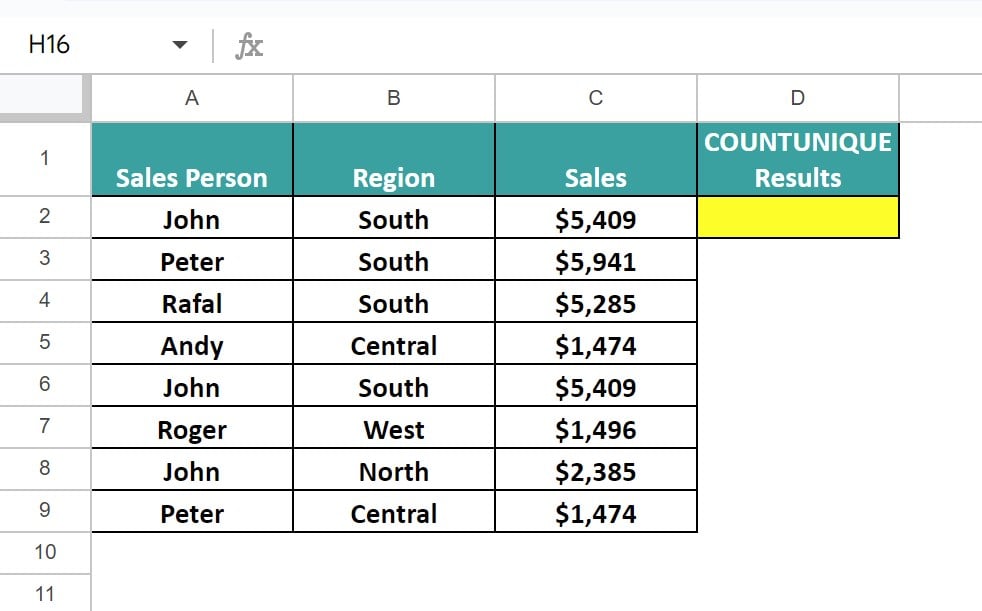
The data of the sales person and their regions and sales is given in the dataset below. We will use the COUNTUNIQUE function to retrieve the unique values countvalues.
The steps to use the COUNTUNIQUE function are,
Step 1: Select cell D2 and enter the formula =COUNTUNIQUE(A1:C9), as shown below.

Step 2: Press “Enter” to get the count of all the unique values ignoring the duplicate values, as shown below.
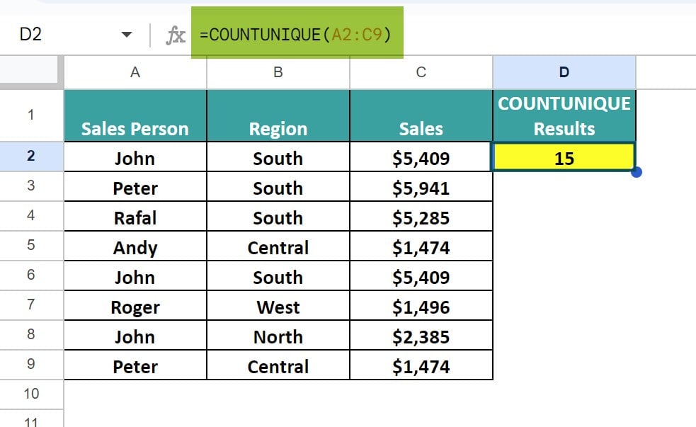
Here, we see the formula counted all the unique values and returned 15, as the result.
Example #2 – Using COUNTNIQUEIFS Function multiple criteria
Let us consider the Example 1 dataset once again where we have the data of the sales person and their regions and sales. We will use the COUNTUNIQUEIFS function to count the unique values that fulfills multiple criterias.

The steps to use the COUNTUNIQUEIFS to satisfy multiple criterias are:
Step 1: Select cell A12 and enter the formula =COUNTUNIQUEIFS(A2:A9,B2:B9,”South”,C2:C9,”>3000″), as shown below.

Step 2: Press “Enter” to get the count of values that satisfy the criterias that the value must be “South” and “>3000” without any duplicate values, as shown below.

In the above image, we have highlighted the four values that satisfy the two criterias, that the value must be “South” and “>3000”. However, one of the four values are repeated, cells B2:C2 and B6:C6. Therefore, the formula ignored the duplicate value and returned the count as 3.
Example #3 – Using COUNTUNIQUEIFS Function single criteria
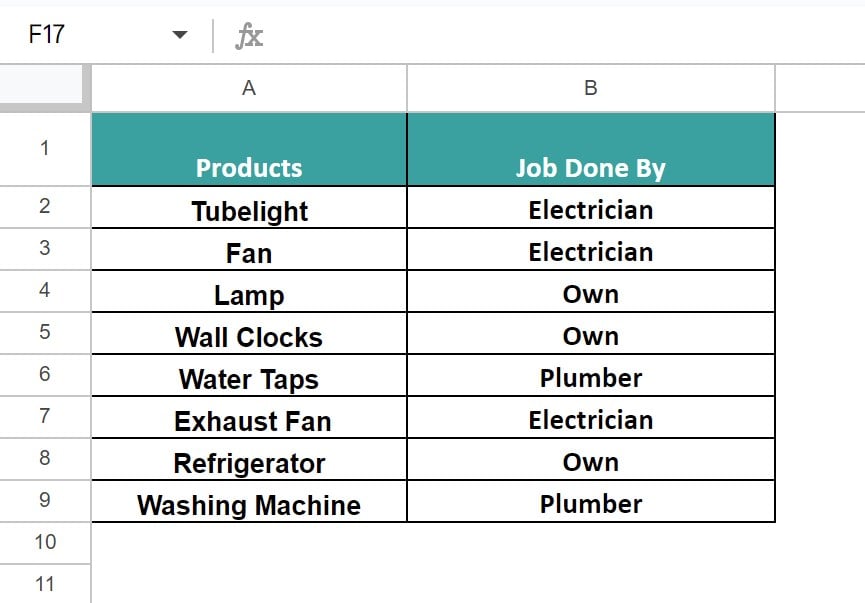
The data consists of some products and the people who fix them. We will use the COUNTUNIQUEIFS formula and find the count of the values that fulfills a single criteria.
The steps to use the COUNTUNIQUEIFS to satisfy single criteria are:
Step 1: Select cell D2 and enter the formula =COUNTUNIQUEIFS(A2:A9,B2:B9,”Plumber”), as shown below.

Step 2: Press “Enter” to get the count of unique values that satisfies the criteria, as shown below.

Example #4 – CountUnique for date values
The data table given below consists of employee names, their ID’s, department, date of Joining, etc. We will count the date values and retrieve the precise count of the unique values.

The steps to count the date values using the COUNTUNIQUE is:
Step 1: Select cell H7 and enter the formula =COUNTUNIQUE(B1:B11), as shown below.

Step 2: Press “Enter”, to get the following data.

We get the result as 4 because there are 4 different dates that are repeated.
Example #5
We have the cosmetics brands campaign data given below with their region and sales. We will use the COUNTUNIQUE function and count the unique values.

The steps to use the COUNTUNIQUE function are:
Step 1: Select cell A8 and enter the formula =COUNTUNIQUE(B2:G5), as shown below.
Here, we will only find the count of unique values of the data entered excluding the horizontal and vertical headers

Step 2: Press “Enter” and we will get the count of the checked data for unique values, as shown below.

Important Things To Note
- Regardless of the dataset size, the COUNTUNIQUE Function will get the count of the unique values, ignoring the duplicates and it will count only once.
- It is case-sensitive. Therefore, ensure to enter the data correctly.
- We get the #REF error if we copy paste the formula in a different worksheet of the same workbook.
Frequently Asked Questions (FAQs)
We often forget in which category a function falls, here, the “COUNTUNIQUE” function. Then, we can insert the function as follows:
Choose an empty cell – select the “Insert” tab – click the “Function” option right arrow -click the “All” option right arrow – select the “COUNTUNIQUE” function, as shown below.
However, as always, entering the function manually is the best way to avoid confusion.
We can insert the COUNTUNIQUEIFS in Google Sheets as follows:
Choose an empty cell for the output – select the “Insert” tab – click the “Function” option right arrow – click the “Statistical” option right arrow – select the “COUNTUNIQUEIFS” function, as shown below.
Alternatively, we can find the Functions icon to insert the COUNTUNIQUE in Google Sheets by following the path shown below.
Choose an empty cell – click the “More” option represented by the three vertical dots at the end of the toolbar, as shown below.
A list of icons appears when we click the “More” option. Here, click the “Functions” icon, as shown below.
Here, click the “Functions” option – click the “All” option right arrow – select the “COUNTUNIQUE” function, as shown below.
The COUNTUNIQUE in Google Sheets is will give an error for the following reasons;
a. The formula is copied form one cell to another and the cell references do not match.
b. The formula argument values are not rightly selected.
c. After the formula is applied and the dataset is modified or deleted, then we will get an error.
Use this COUNTUNIQUE In Google Sheets Template to follow along with the examples in this article.
Download Excel Template