
What Is DATEVALUE In Google Sheets?
The DATEVALUE in Google Sheets converts the date string to the preset date value. The date must be entered as a text within double-quotes and must be in the right date format. The Google Sheets DATEVALUE function helps users to convert selected values into a recognizable format in a large dataset with text format. It also helps to sort, filter, format dates or use in date calculations.
For example, we will find the value of the given date using the Google Sheets DATEVALUE function.

Select cell B2 and enter the formula =DATEVALUE(A2).

The output is shown above as 45583.
Use this DATEVALUE In Google Sheets Template to follow along with the examples in this article.
Download Excel TemplateKey Takeaways
- The DATEVALUE in Google Sheets converts any given valid date, into the preset serial number or its date value. It is used to convert text values containing both dates and times.
- The function has one mandatory argument, i.e., date_string, that has to be a valid date entered within double-quotes or enter the cell reference.
- We can find the date values of the dates by using the DATEVALUE() along with the MID() and FIND() functions in Google Sheets.
- We can perform arithmetic operations such as sum, product, difference, and division, if we have the start_date and the end_date or with the results of the DATEVALUE calculations.
DATEVALUE() Google Sheets Formula
The syntax of the DATEVALUE Google Sheets Formula is,

The mandatory argument of the DATEVALUE Google Sheets Formula is,
- date_string: It is the text that represents the date in proper Google Sheets date format, which is entered in double-quotes.
How To Use DATAVALUE In Google Sheets?
We can use the Google Sheets DATEVALUE function in 2 methods, namely,
- Access from the Google Sheets ribbon.
- Enter in the worksheet manually.
Method #1 – Access from the Google Sheets ribbon –
Choose an empty cell for the output – select the “Insert” tab – click the “Function” option right arrow – click the “Date” option right arrow – select the “DATEVALUE” function, as shown below.

The “DATEVALUE” formula appears, as shown below. Enter the argument value in double-quotes or select the cell reference.

Method #2 – Enter in the worksheet manually –
- Select an empty cell for the output.
- Type =DATEVALUE( in the selected cell. [Alternatively, type =D or =Date and double-click the DATEVALUE function from the list of suggestions shown by Google Sheets.]
- Enter the argument as cell values within double-quotes or cell references.
- Close the brackets and press the “Enter” key.
Examples
We will understand some advanced scenarios with Google Sheets DATEVALUE examples.
Example #1
We will find the date values for dates with different date formats using the Google Sheets DATEVALUE.
In the table, the data is,
- Column A contains the Date.
- Column B displays the Output.

The steps to find the dates using the DATEVALUE function in Google Sheets are,
Step 1: Select cell B2 and enter the formula =DATEVALUE(A2)

Step 2: Press “Enter”. We get the date value as 45319.

Step 3: Drag the formula from cell B2 to B6 using the fill handle to get the following output.

[Note: The first date value in Google Sheets is 31-Dec-1899, unlike Excel’s, which is 1-Jan-1900.]
Example #2
We will calculate the date value using the Google Sheets DATEVALUE function.
In the table, the data is,
- Column A contains the Date.
- Column B contains the Month.
- Column C contains the Year.
- Column D displays the Output.

The procedure to evaluate the dates using the DATEVALUE formula is,
Select cell D2, enter the formula =DATEVALUE(A2&”/”&B2&”/”&C2) and press “Enter”.

The result is “45394”, as shown below.

Example #3
We will calculate the #VALUE! error using the DATEVALUE In Google Sheets formula.
In the table, the data is,
- Column A contains the Date.
- Column B displays the Output.

The procedure to evaluate the dates using the DATEVALUE function in Google Sheets is,
Select cell B2, enter the formula =DATEVALUE(“A2”) and press “Enter”.

The result is a “#VALUE!” error, as shown above, because we entered the arguments cell reference with the double-quotes.
Example #4
We will calculate the difference in date values using the Google Sheets DATEVALUE function.
In the table, the data is,
- Column A contains the DATEVALUE1.
- Column B contains the DATEVALUE2.
- Column C displays the Output of the difference in date values.

The steps to find the difference between the dates using the DATEVALUE() are as follows:
Step 1: Select cell A3, enter the formula =DATEVALUE(A2) and press “Enter”. The result is 45575, as shown below.

Step 2: Select cell B3, enter the formula =DATEVALUE(B2) and press “Enter”. The result is 44572, as shown below.

Step 3: Select cell C2, enter the formula =A2-B2 and press “Enter”.

Step 4: Drag the formula from cell C2 to C3 using the fill handle for further comparison.

The result is “1003”, as shown above. Row 2 is for our reference.
Example #5
The succeeding example depicts the dates with the day. We will calculate the date value by extracting the date from the given data using the DATEVALUE In Google Sheets function with MID and FIND functions.
- The MID function in Google Sheets is a TEXT function that returns a specific number of characters from a text string, starting at the position specified, based on the number of characters specified.
- The FIND function in Google Sheets is a TEXT function that finds the location/position of an alphabet, character or a text string in the selected textual value.
In the table, the data is,
- Column A contains the Date with a space at the start like “ Saturday….
- Column B displays the Output.

The procedure to evaluate the dates using DATEVALUE, MID and FIND formulas is,
Select cell B2, enter the formula=DATEVALUE(MID(A2,FIND(” “,A2)+1,10)) and press “Enter”.

The result is “45584”, as shown below.

Important Things To Note
- Unlike Excel, that gives a #VALUE! error when entering a date value before 1st January 1900, Google sheets gives negative DATEVALUES counting backwards from the preset code such as, 31 December 1899, 30 December 1899, 29 December 1899 & so on as 1, 0, -1 & so on.
- If the start_date exceeds the end_date, then the date value will return a negative number.
- The #VALUE! error occurs,
- When using the DATEVALUE function on earlier dates before December 31, 1899, since this is the first date in Google Sheets with the preset DATEVALUE as 1.
- When the date value or the cell reference is an empty or a blank cell, text value or an alpha-numeric value.
Frequently Asked Questions(FAQs)
We often forget in which category a function falls, here, the “DATEVALUE” function. Then, we can insert the function as follows:
Choose an empty cell -select the “Insert” tab – click the “Function” option right arrow-click the “All” option right arrow – select the “DATEVALUE” function, as shown below.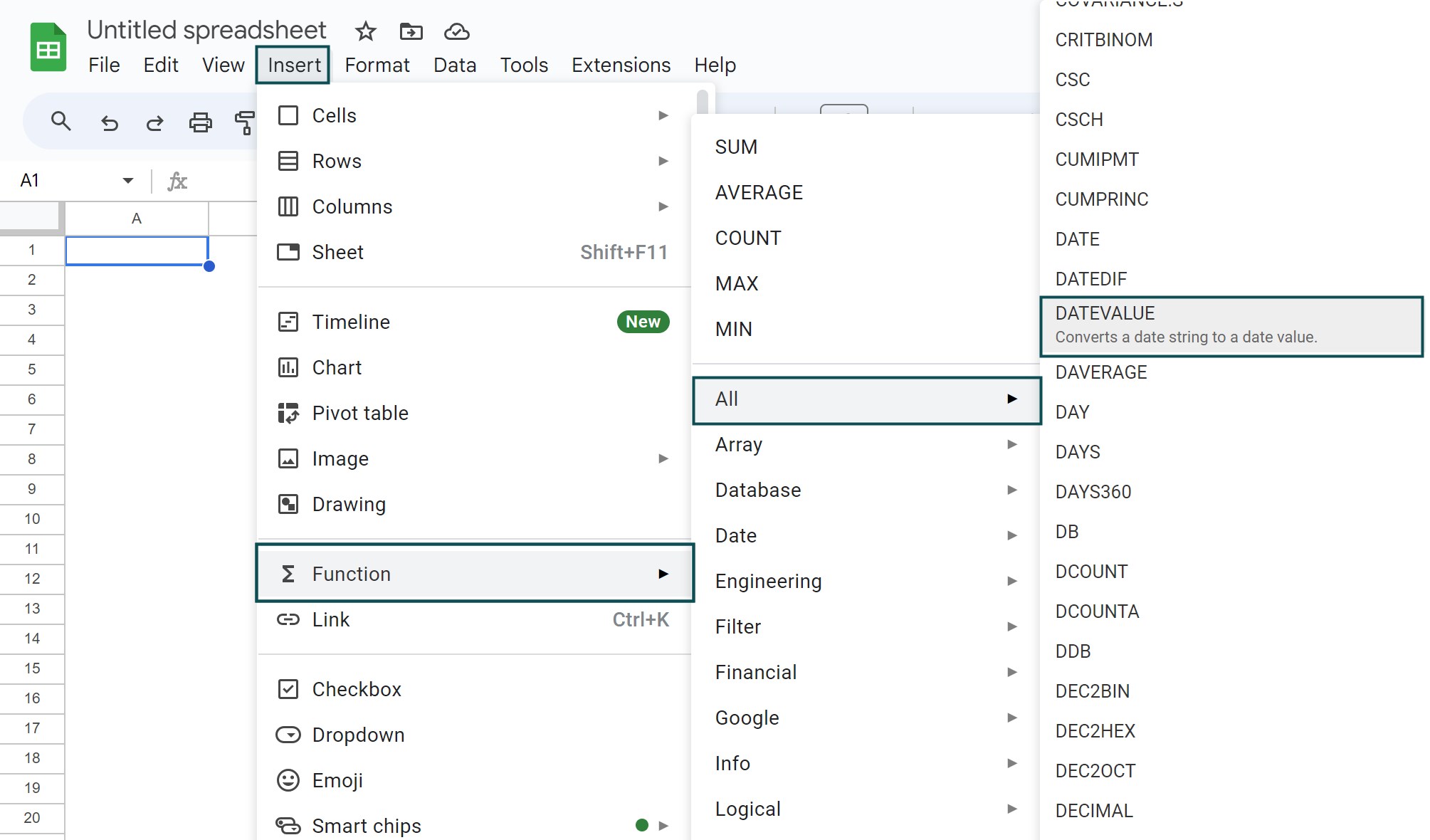
However, as always, entering the function manually is the best way to avoid confusion.
A few reasons the DATEVALUE In Google Sheets function may not work are:
1. The value selected is not in a valid date format.
2. The cell references selected is a text value, alpha-numeric, empty or a blank cell.
3. The dates given is before 31st December 1899 or after 31st December 9999. Also, remember the dates after the last date, i.e., 31st December 9999, can be entered manually, but cannot be selected from the calendar in the Google Sheets as the calendar will be greyed out.
For example, the images below, depicts the last date that can be selected in the Google Sheets in cell A2 and another date that cannot be selected but entered manually in cell A3.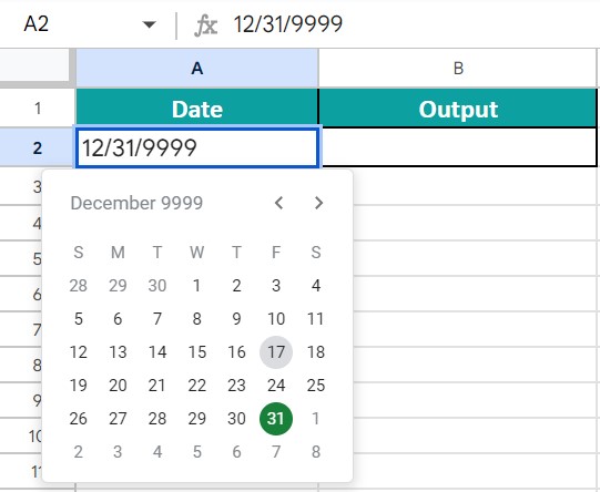
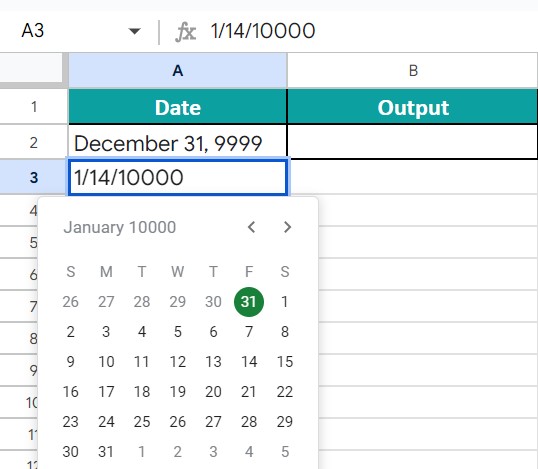
We can see in the 2nd image that, when we hover around the calendar, we are unable to select any date. Hence, entered the date manually.
Now, select cell B2, enter the formula =DATEVALUE(A2), press “Enter” and drag the formula from cell B2 to B3 using the fill handle. We will get the output shown below.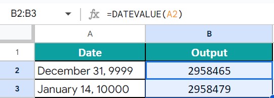
Alternatively, we can find the Functions icon to insert the DATEVALUE function by following the path shown below.
Choose an empty cell – click the “More” option represented by the three vertical dots at the end of the toolbar, as shown below.
A list of icons appears when we click the “More” option. Here, click the “Functions” icon, as shown below.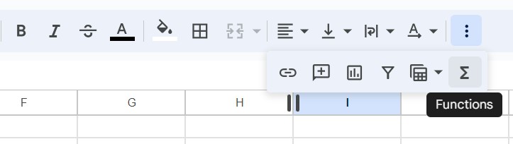
Here, click the “Function” option – click the “All” option right arrow – select the DATEVALUE” function, as shown below.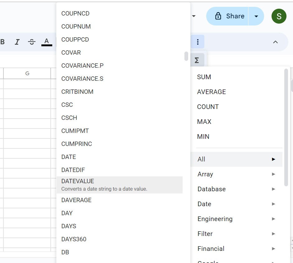
Use this DATEVALUE In Google Sheets Template to follow along with the examples in this article.
Download Excel Template