EDATE in Google Sheets

What is EDATE function in Google Sheets?

There might be instances where we want to find the date that is a specified number of months before or after a given date. We can use the EDATE in Google Sheets to do so. The EDATE function in Google Sheets calculates a date that is a specified number of months before or after a given date. The EDATE function is a powerful tool that can be used for date manipulation. It can be used to forecast revenues, find age, and generate task deadlines in projects. In this article, let us delve into the functionality and capability of the EDATE formula with practical examples to understand it better.

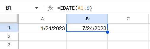
In the example below, we have a date. To find the project’s deadline, which is after 6 months, let us use the following formula.

=EDATE(A1,6).

Here, we get the result of this formula as shown below.

Syntax

Before finding out its applications in detail, let us look at the syntax of the EDATE in the Google Sheets function.

=EDATE(start_date, months)

• start_date: The date from which we want to calculate the result
• months: The number of months before (negative) or the number of months after (positive) the start_date to calculate

How to Use EDATE function in Google Sheets?

As we know, the EDATE function returns a date a specified number of months before or after another date. This formula is helpful when you want to compute a date a particular number of months before or after another date.

There are two ways in which you can insert the EDATE function in Google Sheets.

1. Manually Insert the EDATE function
2. Insert through the Google Menu bar

Manually Insert the EDATE function

Here, we will look at how to insert the EDATE function manually. Let us suppose we are doing some financial reporting. We have a couple of dates. Let us calculate the date two months and six months from the two dates. For this, perform the following steps.

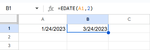
Step 1: Type “=EDATE(” in cell B1.

Step 2: Enter the cell reference containing the date. Here, it is A1. Enter the number of months to add. We add 2 here. Close the braces and press the Enter key.

=EDATE(A1,2).

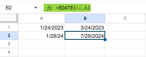
Step 3: Now, drag the formula to cell B2. Change the second argument to 6 as we need the date six months from the supplied date. We get the required dates which are two and six months away from the given dates.

Using the Google Menu bar

1. First, we proceed to the cell where we wish to enter the EDATE formula.
2. In the Google menu bar,  click on “Insert” ➝ “Function” ➝ “DATE” ➝ “EDATE.”
3. Enter the required arguments. Close the bracket and press the “Enter” key.

Examples

The EDATE function in Google Sheets allows us to calculate dates by giving a specified number of months from a given date. This is a useful feature that facilitates calculating the date of completion of various tasks such as forecasting project timelines to managing financial dates. Let us look at some interesting examples on this topic.

Example #1

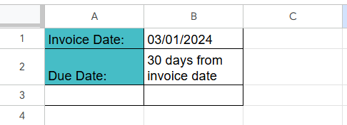
Let us look at a few different ways of using the EDAT function in this example. We have an invoice date for which we must calculate the due date. It is 30 days from the invoice date. Here, we use the EDATE function to calculate the due date.

Step 1: Enter the data in the Google sheet.

• Invoice Date: 03/01/2024
• Due Date: 1 month from the invoice date

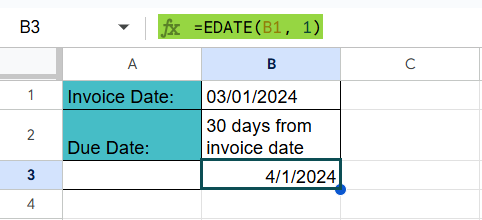
Step 2: Enter the following formula in cell B3.

=EDATE(B1, 1)

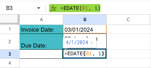
B1 contains the date 01/01/2024 (Invoice Date), and 1 represents adding one month. Press Enter. You get the result as 4/1/2024.

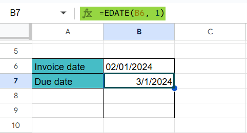
Step 3: Let us check what happens if the scenario is a leap year. Enter the new invoice date as 02/01/24. Use the EDATE function in B6 as shown below.

=EDATE(B6,1). Press Enter. As 2024 is a leap year, it also maintains the last day of February.

To compute the last day of the month returned by EDATE, use the EOMONTH function as shown below. ==EOMONTH(B6, 1)

Example #2 – Schedule for Subscription Renewals

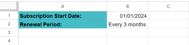
Suppose you have a Netflix subscription that renews every 3 months. In such a scenario, it is very simple to calculate the renewal dates based on the subscription date using EDATE in Google Sheets.

Step 1: Enter the details in a sheet as shown below.

• Subscription Start Date: 01/01/2024
• Renewal Period: Every 3 months

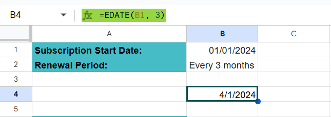
Step 2: Let us enter the formula to calculate the next renewal date. Enter the following formula in cell B4.

=EDATE(B1, 3)

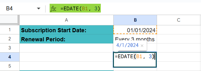
Step 3: Press Enter. You get the result as 04/01/2024.

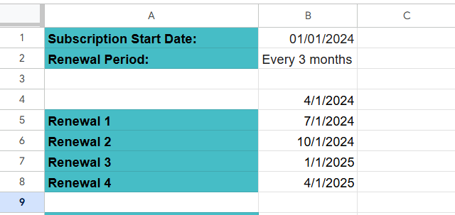
Instead of calculating the renewal date each time manually, you can use this formula and drag it to calculate the renewal dates for subsequent years.

While using EDATE in Google Sheets, always be cautious to ensure the date input to the function is either a cell reference of a date, a function that returns a date such as DATE, or a date serial number.

Now, before we proceed to the next example, let us try to calculate the previous renewal date, before the first supplied date. For this, you can use EDATE with a negative value to subtract months.

Step 4: Enter the following formula in B10.

=EDATE(B1, -3). Press Enter.

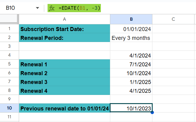
The previous renewal date will be 10/01/2023.

Example #3 – Combining EDATE with WEEKDAY Function

Suppose a worker is working with some products in a supermarket that has an expiry date of 2 months from the shelf life of the manufacturing date. He can only restock and remove old stock on a weekday. So, he finds out if the expiry date is a weekday so that he can get it removed prior if it isn’t. In this case, you can use EDATE along with WEEKDAY to calculate the expiry date and day.

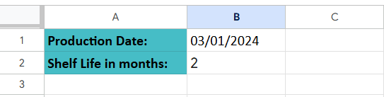
Step 1: Enter all the details in a sheet.

• Production Date: 03/01/2024
• Shelf Life in months: 2

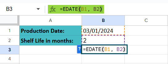
Step 2: Enter the following formula for the expiry date.

=EDATE(B1, B2). Press Enter.

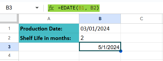
Step 3: The expiry date will be 05/01/2025.

Now, to get the weekday of the expiry date, wrap the formula in WEEKDAY.

=WEEKDAY(EDATE(B1, B2)). Press Enter.

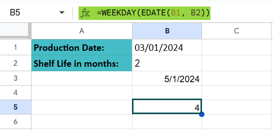
You get the WEEKDAY as 4, indicating that the worker can remove the product a day prior as it is not a weekend.

By combining EDATE with WEEKDAY in Google Sheets, you can create dynamic date calculations that help manage scheduling, deadlines, and time-sensitive events.

Important Things to Note

1. If the argument start_date is not a valid date, the EDATE function returns a #VALUE! Error.
2. If the months argument is not an integer, the decimal part is truncated, and the number is treated as a whole number.
3. The EDATE function returns a serial number corresponding to the date (General format). For the result to display correctly, it must be formatted as a date.

Frequently Asked Questions (FAQs)

Download Template

This article must help understand EDATE in Google Sheets with its formulas and examples. You can download the template here to use it instantly.

Recommended Articles

Guide to What Is EDATE in Google Sheets. We learn its syntax & how to use it to find a specific date with examples and a working template. You can learn more from the following articles. –

Gantt Chart in Google Sheets

COUNTBLANK In Google Sheets

Insert Comment In Google Sheets