
What Is EXACT In Google Sheets?
EXACT function in Google sheets, as the name suggests, helps users compare and find if the text string is exactly the same. It is a default inbuilt function available in both Excel and Google sheets.
Remember, users can use EXACT function to compare two string values from the data. We need to make sure that the EXACT function is case-sensitive and therefore, text in uppercase and lower-case text strings will be considered differently.
Use this EXACT In Google Sheets Template to follow along with the examples in this article.
Download Excel TemplateFor example, consider the below table showing ‘APPLE’ in uppercase letters in column A.

Now, we need to use the EXACT function to find whether the text is exactly the same.
To begin with, select the cell B2 and insert the EXACT function formula =EXACT(A2,”Apple”). Press Enter key.
We will be able to see the result, as shown in the below image.

Likewise, we can use the EXACT function to find and compare if the text is same or not.
In this article, let us learn how to use the EXACT function with the help of detailed following examples.
Key Takeaways
- EXACT function in Google sheets, in simple terms, is used to find whether the data is exactly the same in the given cell.
- The syntax of the EXACT function in Google sheets is =EXACT(string1,string2,…) where string1 is the first value to be checked and compared.
- Similarly, string2 is the second string to be compared and analyzed in the formula.
- Remember, the EXACT Google sheets function is case-sensitive and we need to make sure the data is correct as mentioned in the syntax.
Syntax

The formula or syntax of EXACT function is =EXACT(string1,string2,…)
where,
- string1 is the first value to be checked and compared
- string2 is the second string to be compared and analyzed
How To Use EXACT In Google Sheets?
We can use EXACT function in Google sheets in two different methods. They are:
- Selecting the EXACT function under the Insert tab
- Manually typing the EXACT function
Method #1 – Selecting the EXACT function under the Insert tab
The steps to select the EXACT function under the Insert tab are:
Step 1: To begin with, we need to insert the data in the Google spreadsheets. Next, we need to select the cell where we want to find the result.
Step 2: Next, select the Insert tab. Then, click on the Function option.
Step 3: Now, click on the Text category options. Click on EXACT function.

Step 4: We will be able to see the EXACT function formula in Google sheets. Now, select the arguments required in the formula.
Step 5: Press Enter key. We will be able to see the result in the active cell.
Likewise, we can use the EXACT function under the Insert tab.
Method #2 – Manually typing the EXACT Function
The steps to select the EXACT function in Google sheets manually are:
Step 1: To begin with, we need to insert the data in the Google spreadsheets. Next, we need to select the cell where we want to find the result.
Step 2: Next, enter =EX. Then click on EXACT function in the drop-down list.

Step 3: Alternatively, manually type =EXACT directly.
Step 4: We will be able to see the EXACT function formula. Now, select the arguments required in the formula.
Step 5: Press Enter key. We will be able to see the result in the active cell.
Likewise, we can use the EXACT function in Google sheets manually.
Examples
Now, let us learn how to use the EXACT function with the help of following examples.
Example #1
For example, consider the below table showing names of an individual in different formats in uppercase, proper case etc in column A.

Now, we need to use the EXACT function to find whether the text is exactly the same as ‘Andy’.
The steps to select the EXACT function are:
Step 1: To begin with, we need to insert the data in the Google spreadsheets. In this example, the data is available in the cell range A1:B5. Next, we need to select the cell where we want to find the result. In this example, we need to select the cell B2.
Step 2: Next, select the EXACT function in Google sheets.
So, the complete formula is =EXACT(A2,”Andy”)

Step 3: Press Enter key.
We will be able to see the result in cell B2, as shown in the below image.

Now, using the AutoFill option, we will be able to see the result in the cell range B3:B5, as shown in the below image.

Note that the result shows FALSE in cell range B2:B4 and TRUE in cell B5, as EXACT function is case-sensitive and considers same text string in upper case, lower case, and proper case as differently.
Likewise, we can use the EXACT function to find whether the data is exact or not.
Example #2 – Combining EXACT With Conditional Formatting
For example, consider the below table showing regions in uppercase, proper case etc in column A.

Now, we need to use the EXACT function to find whether the text is exactly the same as ‘North.
The steps to select the EXACT function are:
Step 1: To begin with, we need to insert the data in the Google spreadsheets. In this example, the data is available in the cell range A1:A5. Next, we need to select the cell range which we want to find the exact value using conditional formatting. In this example, we need to select the cell range A1:A5.
Step 2: Next, select the Format tab and click on Conditional Formatting.
Step 3: The Conditional Format Rules tab appears at the right end of the screen. Go to the next step.
Step 4: Now, select the Format cells if under the Format rules option and select Text is exactly.
And enter the value as North.

Step 5: Now, we will be able to see the result in the cell range A2:A5, as shown in the below image.

Likewise, we can find whether the data is exact or not using the conditional formatting tab.
Example #3 – Integrating EXACT With IF Statements
For example, consider the below table showing region, status, completed and result in columns A, B, C and D, respectively.

Now, we need to use the EXACT function in Google sheets with IF function.
The steps to select the EXACT function in Google sheets are:
Step 1: To begin with, we need to insert the data in the Google spreadsheets. In this example, the data is available in the cell range A1:D4. Next, we need to select the cell where we want to find the result. In this example, we need to select the cell D2.
Step 2: Next, select the EXACT function.
So, the complete formula is =IF(EXACT(B2,”Declined”),0,C2)

Step 3: Press Enter key.
We will be able to see the result in cell D2, as shown in the below image.

Now, using the AutoFill option, we will be able to see the result in the cell range D3:D4, as shown in the below image.

Likewise, we can use the EXACT function with IF function to find whether the data is exact or not.
Example #4 – Combining EXACT With Arrayformula
For better understanding, let us use the same example we used in Example 1. Consider the below table showing names of an individual in different formats in uppercase, proper case etc in column A.

Now, we need to use the EXACT function to find whether the text is exactly the same as ‘Andy’.
The steps to select the EXACT function are:
Step 1: To begin with, we need to insert the data in the Google spreadsheets. In this example, the data is available in the cell range A1:B5. Next, we need to select the cell where we want to find the result. In this example, we need to select the cell B2.
Step 2: Next, select the EXACT function with ARRAYFORMULA function.
So, the complete formula is =ARRAYFORMULA(EXACT(A2,”Andy”))

Step 3: Press Enter key.
We will be able to see the result in cell B2:B5, as shown in the below image.

Likewise, we can use the EXACT function with ARRAYFORMULA to find whether the data is exact or not.
Important Things To Note
- EXACT function is a default function used to find whether the data is same.
- The data in a particular cell can be checked using the EXACT function in Google sheets.
- Remember, to check an entire cell range without using the Autofill option, we can use the ARRAYFORMULA with EXACT function.
Frequently Asked Questions (FAQs)
For example, consider the below table showing names of an individual in different formats in uppercase, proper case etc in column A.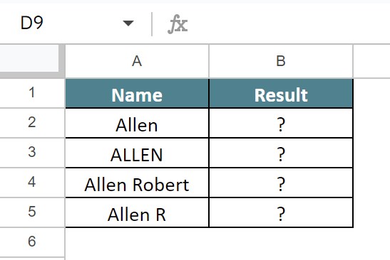
Now, we need to use the EXACT function to find whether the text is exactly the same as ‘Allen’.
The steps to select the EXACT function in Google sheets are:
Step 1: To begin with, we need to insert the data in the Google spreadsheets. In this example, the data is available in the cell range A1:B5. Next, we need to select the cell where we want to find the result. In this example, we need to select the cell B2.
Step 2: Next, select the EXACT function.
So, the complete formula is =EXACT(A2,”Allen”)
Step 3: Press Enter key.
We will be able to see the result in cell B2.
Now, using the AutoFill option, we will be able to see the result in the cell range B3:B5, as shown in the below image.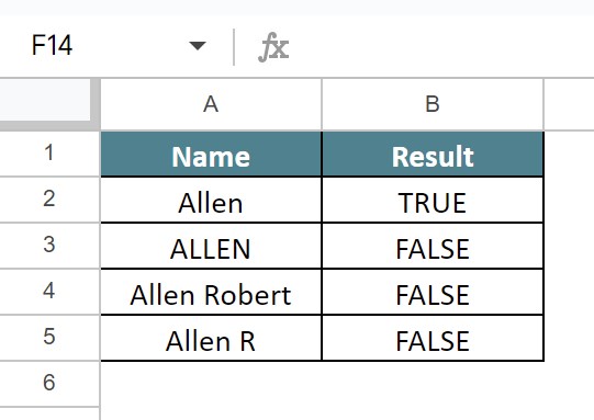
Note that the result shows FALSE in cell range B3:B5 and TRUE in cell B2, as EXACT function is case-sensitive and considers same text string in upper case, lower case, and proper case as differently.
Likewise, we can use the EXACT function to find whether the data is exact or not.
EXACT function in Google sheets may not work
• If the number of required arguments is less or more
• If the data does not match with the arguments
EXACT function can be nested with other functions such as IF function in Google sheets. Similarly, we can also use EXACT function with conditional formatting in Google sheets.
Use this EXACT In Google Sheets Template to follow along with the examples in this article.
Download Excel Template