
What Is Conditional Formatting In Google Sheets?
Conditional formatting in Google Sheets allows you to change the formatting of cells that meet a specific criterion. You can apply conditional formatting to a specific row, column, or even a cell based on some set of rules you have given. This feature helps your data in Google Sheets be noticeable more based on specific conditions.
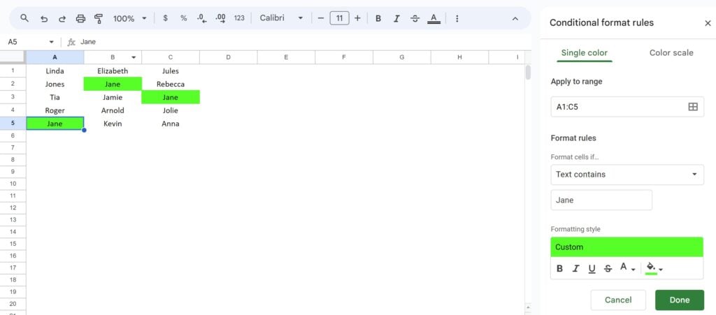
For instance, in the example below, we used conditional formatting to apply a green color to all the cells containing the text “Jane.” As you can see, we have the “Conditional format rules” pane open when we go to the Format tab-> Conditional Formatting and set rules accordingly.
Use this Conditional Formatting In Google Sheets Template to follow along with the examples in this article.
Download Excel TemplateKey Takeaways
- Highlighting data with color based on certain conditions such as greater or lesser than some value, or containing certain characters, can be done through conditional formatting. Using this option, we change the font, font color, or background color according to specified rules. This will be applied automatically to the range specified.
- To apply conditional formatting, go to the Format menu item and click on Conditional formatting. The “Conditional format rules” pane opens where we can set rules accordingly.
- Google Sheets conditional formatting based on another cell can be done by just using your own formula with a reference to the cell where you specify the necessary condition.
- You can use the color scale to apply conditional formatting not only with one hue but using a color scale. You can pick hues for the minimum and maximum points, as well as for the midpoint.
How To Access Conditional Formatting In Google Sheets?
To access conditional formatting,
- Open the required spreadsheet in Google Sheets.
- Select the range that you want to format. For example, cells A2:B10
- Click on the Format tab. In that, select Conditional formatting.
- Under the “Format cells if” drop-down, click the option “Custom formula is.” …
- Write the required rules.
- You can choose different formatting properties.
- Click Done.
How To Use Conditional Formatting In Google Sheets?
Interpreting a Google sheet with data is easy if we have less data in it. However, when it comes to spreadsheets full of data, it is not everyone’s cup of tea to understand or summarize the critical points in the data at a glance. Here’s where conditional formatting comes to your rescue. You can set specific conditions for which formatting can be done according to requirements to highlight particular data of choice.
While this sounds complicated, it is simple.
Step 1: To access conditional formatting for the sheet below, first select the data and go to the Format tab.

Step 2: In the Format tab, choose the “Conditional Formatting” option.

Step 3: In the ‘Conditional Format rules” side panel, the desired range is already mentioned as we have selected it. Under the “Format cells if” drop-down menu, there are plenty of options, as seen below.

Step 4: Here, we plan to find the top students by highlighting their cells in green. Choose the option “Text is exactly,” and type “A” in the box below.

Step 5: Choose the color for the cells and press “Done.”

Step 6: Now, the cells with Grade A are highlighted. From this, you get an idea of the top students.

Under Formatting style, select your formatting style. You can choose other formatting properties.
Suppose you are viewing a highlighted sheet; you can open the Conditional format rules following the first step above, which will display a complete list of the existing rules. You can remove rules by clicking on the “Trash bin” icon.

Advanced Conditional Formatting Usage
Advanced conditional formatting allows you to format cells based on complex formulas and conditions and where the values can be present in different locations in Google Sheets. The criteria for conditional formatting can be set to different locations under Google Sheets conditional formatting multiple conditions as well. To understand this further, let us look at some interesting examples.
Example #1 – Create New Rules
With the effective conditional formatting available in Google sheets, you can not only do formatting for some simple rules, but also create new rules which can be simple or complex. Let us look at an example. In the sheet below, we have the rainfall in a few cities for the months ranging from Jan-March.

Step 1: To apply a new conditional formatting rule, let us go to Format->Conditional Formatting.

Step 2: You get the “Conditional Format rules” panel on the left side. Click on “+Add another rule.”

Step 3: Select the required range where you want to apply the formatting under “Apply to Range.”

Step 4: Under the option “Format cells if..” choose the required condition, choose “Less than,” and add the number 10. Here, we are going to display rainfall less than 10 mm, between 10 mm and 20 mm, and greater than 20 mm in different shades.
First, we choose the option “Less than” and enter the number 10. Under Formatting Style, choose a shade of your choice.

Step 5: Now, press the option “Add another rule” below the option “Done.”

Step 6: Repeat the same steps as above, choosing the option “greater than” and a shade for it.

Step 7: Finally, repeat the same for values between 10 and 20, as shown.

Step 8: Press Done. You can see all the rules set in the side panel. Now, look at the data.
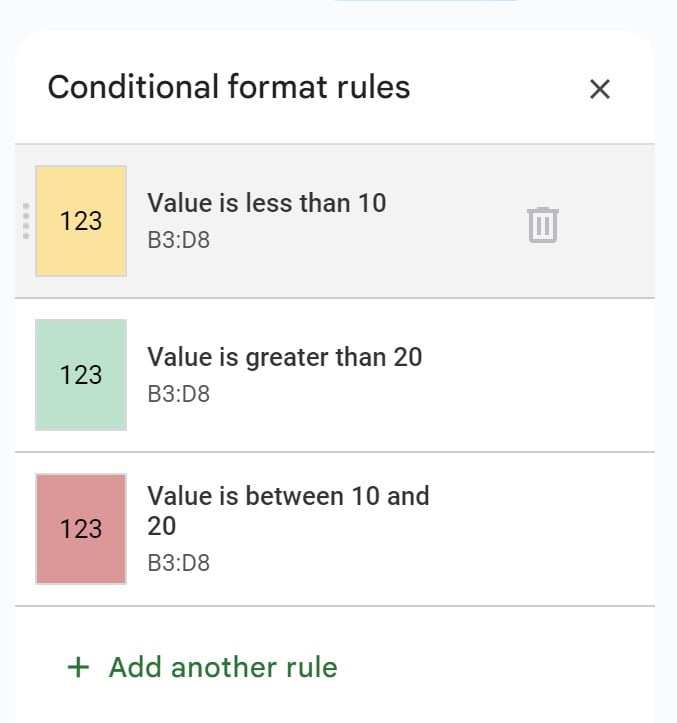
The table helps us quickly determine the pattern of rainfall in these cities, thereby helping us make informed decisions.

Example #2 – Based on Cell Value
Let us look at another example where we highlight rows based on a cell value. We have some store sales details.

Step 1: Let us highlight the entire row based on the sales value. Here, we highlight the entire row for all sales greater than 80.
Go to Format-Conditional Formatting and click on “Add another rule.”

Step 2: To highlight the entire row in the range for all sales > 80, enter the range you want to apply this formula to.

Step 3: Choose Custom formula is under the “Format cells if..” option. With this, you can apply Google Sheets conditional formatting custom formula.

Step 4: Here, if we choose the option greater than, only the individual cell is highlighted. We want to highlight the entire row whose sales are greater than 80. Enter the following formula in the box.
=($B2>80) and choose a custom color under formatting style.

Step 5: Press Done. You can see the entire row highlighted based on the cell values in Column B greater than 80.

Example #3 – Multiple Conditional Formatting Rules in One Cell/Table
When applying conditional formatting in Google Sheets, you must understand that you are not restricted to one rule per cell. You can apply as many rules as you require. You can apply a rule and then another on the same range. The order in which the rule appears is the order of precedence.
For example, you can create two rules to highlight the numbers that are even in one color and less than 50 in another color. However, for the rules to work correctly, the order in which they are arranged is essential. For instance, if the even number property is added first and the less than 50 rule next, even if the number is both even and less than 50, the even number rule color will be applied due to its order of precedence.
Let us demonstrate it in Google sheets.
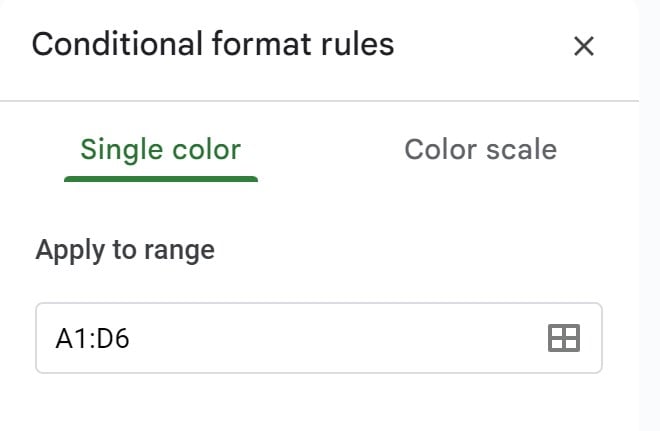
Step 1: Look at the table below. Click on Format – Conditional Formatting. You get the side panel called “Conditional Format rules.”

Step 2: You can start adding the two rules. First, let us change the color of number less than 50. For this, first, enter the range where the numbers are present.

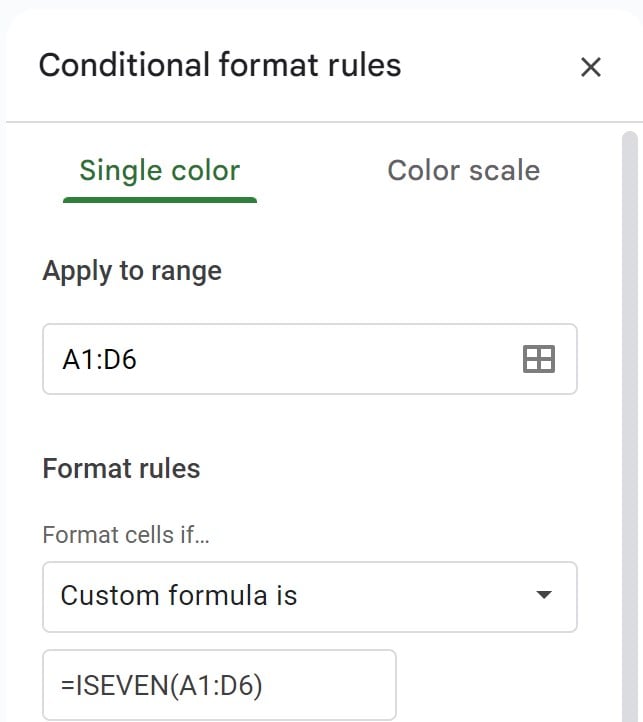
Step 3: Under “Format Rules,” choose the option “Custom formula is.”

Step 4: In the box below, enter the formula. Here, we are checking for the even numbers first. So, enter the formula as you would in any Google sheet cell. Here, we enter =ISEVEN(A1:D6) and choose the required color.

Step 5: Press Done. You have the first rule ready!

Step 6: Now, click on “Add another rule.” Choose the option “Less than” under “Format cells if” and apply the desired color.

Step 7: You can now see the two different rules applied to the same range. Observe the table and see how the colors have been applied. Red is for the even numbers, and green is for numbers less than 50.

If you observe, the rules have been applied in the order in which they are set. 22 in cell B3, is less than 50, and even. However, the even rule is applied first here, and the number is in red. The cells which do not fulfil both rules are still in black.
How To Edit Conditional Formatting Rules?
In Google Sheets, you can edit an existing rule that you have set for a range or change the formatting.
Step 1: It is as simple as it gets. Considering the previous example, first select the formatting range. In the Menu, go to Format – Conditional Formatting.

Step 2: The Conditional format rules pane opens on the right side of the sheet. Double-click on the rule you want to edit.

Step 3: You can edit the rule and click Done.
Copy Conditional Formatting Rules
Sometimes, it is required to copy the formatting of a range to another cell/range. In such cases, Google Sheets offers you an easy solution.
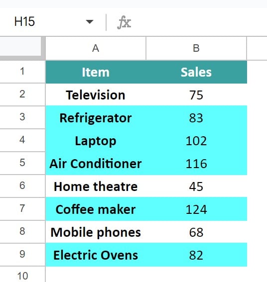
Consider this sheet from the early example. Here, we have highlighted all the rows where the sales are greater than 80.

Step 1: Let us enter a few more items. As seen below, these rules have not been applied to the new entries as they are outside the specified range(A2:B5).

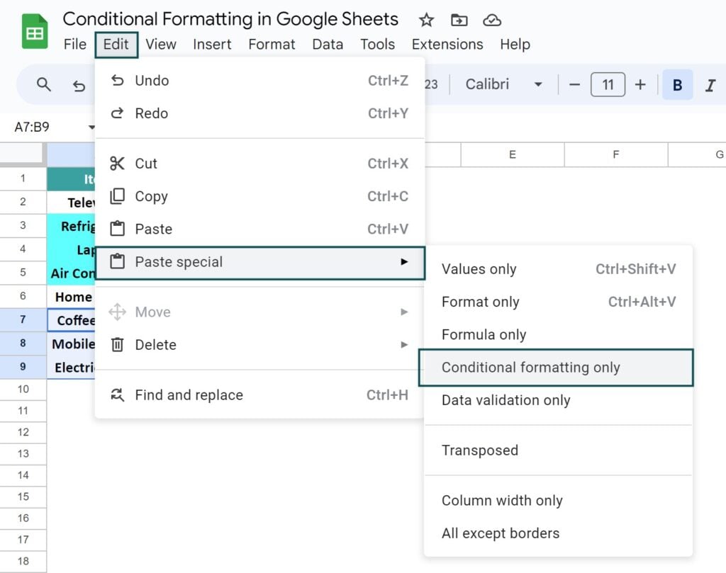
Step 2: To copy the formatting, first select the initial range(A2:B5) and go to Edit – Copy.

Step 3: Now, select the target range, A7 to B9.

Step 4: Go to Edit – Paste Special. Choose the option “Conditional Formatting only.”
You can see that the formatting for highlighting sales greater than 80 is applied here.
Important Things To Note
- The various options available under “Format cells if..” in the “Conditional format rules” pane, including adding custom formulas, make it highly comprehensive to add any formatting to a range/cell.
- The Past Special option under the Edit tab helps you copy-paste only the formatting of cells, leaving out the data.
- You can use the Color Scale feature to create Heatmaps in Google Sheets.
- If your cell contains values like numbers or dates, you can specify a minimum, maximum, or range of values to be highlighted in Google Sheets.
Frequently Asked Questions (FAQs)
Automatically applying conditional formatting is simple. Highlight the range where you want to apply it, click Format > Conditional formatting, and then click Add another rule. Google Sheets will run through each rule according to their order until it satisfies a condition that requires a change in style.
Sometimes when applying conditional formatting, you may not apply it to all the cells you want it to. Hence, check the range in ‘Apply to range’ in the Conditional format rules pane and make sure you have specified the range separated by a colon, such as A1:A15.
In Google Sheets, the conditional format rules only apply to the tab they are entered on. You can’t import them onto multiple tabs at the same time. However, you can copy the conditional formatting from a range in a sheet and apply it to the desired range of another sheet individually.
Use this Conditional Formatting In Google Sheets Template to follow along with the examples in this article.
Download Excel Template