What Are Advanced Google Sheets Formulas?
The advanced Google Sheets formulas are expressions created using inbuilt functions, arithmetic operators, and given data, to perform complex evaluations quickly.
Users can utilize the advanced Google Sheets formulas to make data updates, maintenance, and manipulation in the spreadsheet application highly effective and organized. Also, the formulas help in automating complicated calculations, which ensures improved data accuracy and quality.
For example, the source dataset contains employees’ first and last names.

We must combine the first and last names of each employee to display their full names in the corresponding column C cells.
Then, we can apply the Google Sheets advanced formulas and functions, such as the CONCATENATE or CONCAT, in the target cells to secure the required outcome.

In this example, we use one of the concatenation Google Sheets advanced formulas and functions, CONCATENATE.
The function accepts three argument values. The first one is a reference to the cell holding an employee’s first name, the second is a space character, and the third is a reference to the cell holding the employee’s last name.
The function then combines the input values to return the concerned employee’s full name. Please note that if we do not supply the space character after the first name, the function will concatenate the first and last names without a space.
Table of contents
Key Takeaways
- The advanced Google Sheets formulas are powerful data evaluation tools that help perform complex computations quickly and accurately. While they manage multiple calculation steps in the backend, they help automate mathematical evaluations that we might repeatedly use during our spreadsheet-based activities.
- The advanced formulas in Google Sheets help in entering, updating and manipulating massive datasets error-free.
- Though the advanced formulas in Google Sheets are highly efficient, we must adhere to the defined functions’ syntaxes to ensure they return the correct output.
- Though we can apply different advanced formulas in Google Sheets individually, using them with other inbuilt functions makes them highly practical.
List Of Top 10 Advanced Google Sheets Formulas
The following are the top ten advanced Google Sheets formulas that we will find useful in our daily spreadsheet-based tasks.
#1 – VLOOKUP Formula In Google Sheets
The VLOOKUP is one of the most useful advanced Google Sheets formulas.
The function helps look for the given search key value in the first column of the specified lookup range. Next, once it finds a match for the search key in the specific column, the function returns the value in the corresponding row of the column, indicated by the specified index.
Please note that the column holding the return values will be on the right of the first column in the lookup range, with the index value denoting its position in the lookup range. Also, the match can be exact or approximate.
For example, the first dataset contains the top ten firms and their financial details. Next, the second dataset lists the stock names and their respective company’s revenue.
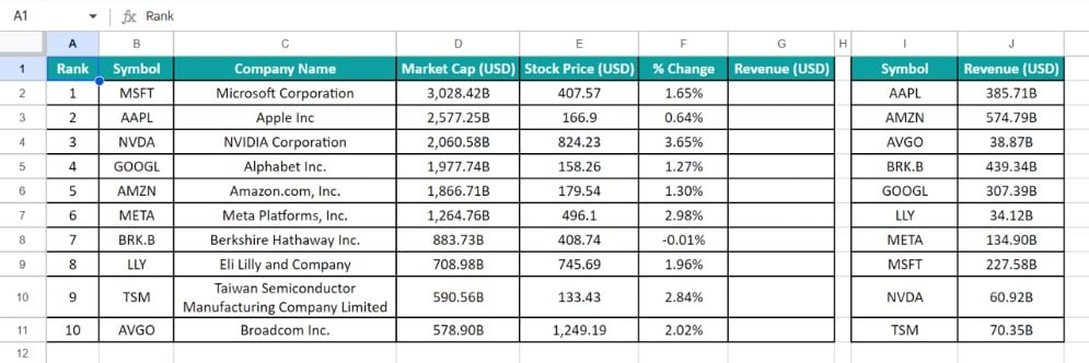
We must update the revenue data for the listed companies in column G of the first dataset based on the second dataset.
Then, we can utilize useful advanced Google Sheets formulas such as the VLOOKUP(), which works like the Excel VLOOKUP function, in column G cells to fetch the required output.
Step 1: Choose cell G2 and enter the VLOOKUP().

Step 2: Provide the argument values, separated by commas, close the brackets, and press Enter.
=VLOOKUP(B2,$I$2:$J$11,2,0)
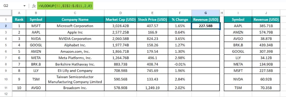
Step 3: Use the fill handle to feed the function in the remaining target cells.
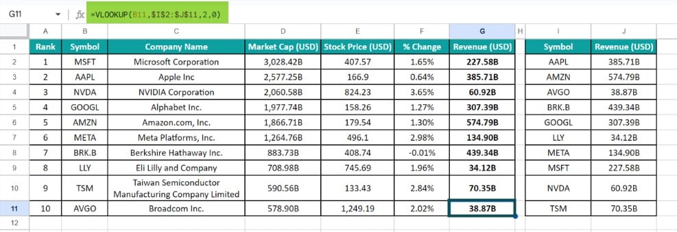
Let us check the cell G11 formula to know the logic.
The VLOOKUP() accepts four argument values as input. The first is the reference to the cell B11 containing the search key AVGO. Next, the lookup range is I2:J11, which we supply as an absolute reference. The reason is that the lookup range is constant in all the target cells’ formulas, and it helps apply the formula with minimum modifications in the rest of the target cells. Next, the specified column index value is 2, indicating that the function should return the output value from the second column of the lookup range. Finally, the last argument value of 0 denotes that the function must find an exact match for the search key in the lookup range.
So, the function finds the exact match for the search key AVGO in cell I4. Thus, the function returns the value in row 4 of column J, which is the cell J4 value of 38.87B.
#2 – INDEX Formula In Google Sheets
The INDEX function-based advanced Google Sheets formulas return a value or a cell reference to the value fetched from the specified cell range. We must provide the rows and columns-based dimensions as inputs to the function.
For example, the source dataset lists US cities, the median home prices and monthly rents, and the average yearly salaries in the listed cities.
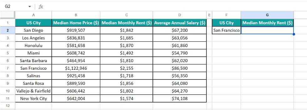
The aim is to determine the median monthly rent for the US city cited in cell F2. Assume the target cell is G2.
Then, we can apply the INDEX(), which works like the Excel INDEX function, in the target cell to acquire the required value.
Step 1: Select cell G2 and enter the INDEX().

Step 2: Update the argument values, separated by commas, close the brackets, and press Enter.
=INDEX(A2:D11,6,3)
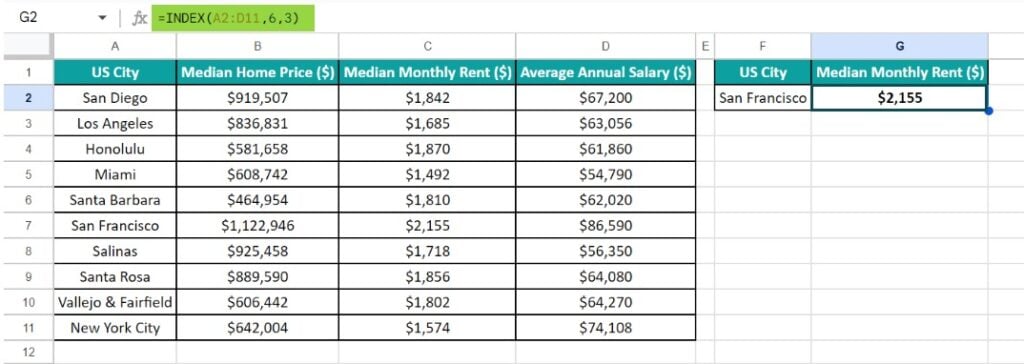
The INDEX() accepts three argument values. The first is the reference range A2:D11, from where we must get the required data for the US city of San Francisco, cited in cell F2. Next, since the specified city is in row 6 of the range A2:D11, the second argument value is 6. Further, since we count the rows from row 2 of the sheet, the actual row we must refer to is row 7 of the sheet. Next, the third argument value is 3 since we must fetch the required data from the third column, column C, of the reference range.
Thus, for the input values, the function returns the cell C7 value of $2,155.
#3 – MATCH Formula In Google Sheets
The MATCH function-based advanced Google Sheets formulas return the relative position of the given item in the specified cell range. Further, the function can find an exact or approximate match for the specified item, which we must specify while supplying the inputs to the function.
For example, the source dataset contains the top ten tech companies and their stock prices.
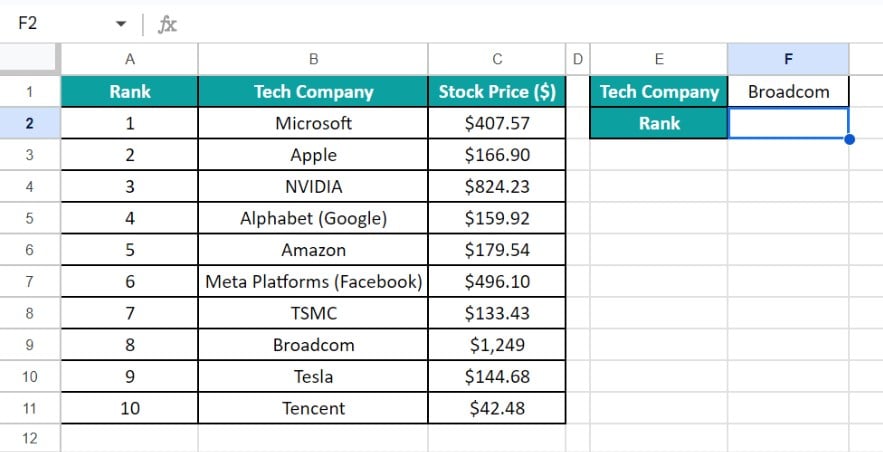
The requirement is to determine the rank of the company given in cell F1 and show the outcome in cell F2.
Step 1: Select cell F2 and enter the MATCH(), which works like the Excel MATCH function.

Step 2: Update the argument values, separated by commas, close the brackets, and press Enter.
=MATCH(F1,B2:B11,0)

The MATCH() takes three argument values as input. The first argument value is the reference to cell F1 containing the search key Broadcom. Next, the second argument value is the search range B2:B11, where the function must look for the search key. Next, since we need an exact match for the search key in the cited range, the third argument value is 0.
So, the function finds an exact match for the given company name Broadcom in cell B9. Thus, the function returns the relative position of cell B9 in the range B2:B11 as the required rank, which is 8.
#4 – XLOOKUP Formula In Google Sheets
The VLOOKUP() is one of the most helpful advanced Google Sheets formulas explained previously.
However, the XLOOKUP(), which works like the Excel XLOOKUP function, is a more practical alternative.
The function searches for an item in a lookup range and determines the row where it finds the match. It then returns the value in the corresponding row of the specified column, which holds the potential return values.
Furthermore, the function allows us to specify inputs to indicate the required match and search modes. Also, we can mention the text to display in the case when the function does not find a match for the search key.
For example, the source dataset contains a firm’s invoice data.

The requirement is to update the units ordered data for the invoice number cited in cell G1 and display the target data in cell G2.
Then, we may plan to use the VLOOKUP(), which is one of the most widely used advanced Google Sheets formulas explained previously.
However, a more efficient option is to use the XLOOKUP() in the target cell. The reason is that the function will work even when the return value range is on the left of the lookup column.
Step 1: Select cell G2 and enter the XLOOKUP().
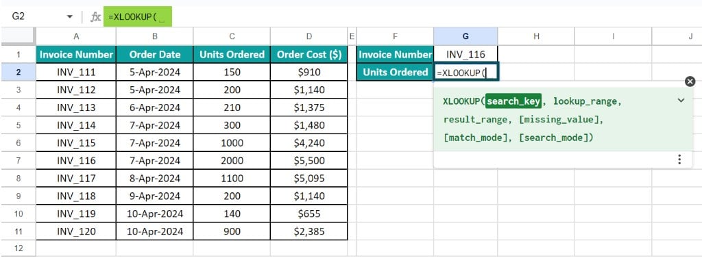
Step 2: Supply the argument values, separated by commas, close the brackets, and press Enter.
=XLOOKUP(G1,A2:A11,C2:C11)

The XLOOKUP() accepts three argument values as input. The first argument is the reference to cell G1 holding the search key value INV_116. Next is the lookup range A2:A11, where the function must look for a match for the search key. After that, the third argument is the return value range C2:C11, holding the potential return values. Furthermore, we did not mention the match and search mode values. So, the function takes their default values and looks for an exact match for the cited search key value from the top cell in the lookup range.
So, the function looks for an exact match for the invoice number INV_116 in the lookup range A2:A11, which it finds in cell A7. Thus, it returns the value in row 7 of the return value column range C2:C11, which is the cell C7 value of 2000, as the required units ordered value.
#5 – IF AND Formula In Google Sheets
The IF-AND formula is an IF(), which uses the AND() in its condition to check multiple criteria in one go. The function then returns the TRUE value only when all the specified conditions are met. Otherwise, it returns the cited FALSE value.
For instance, the source dataset lists stationery items and their store-wise units available data.
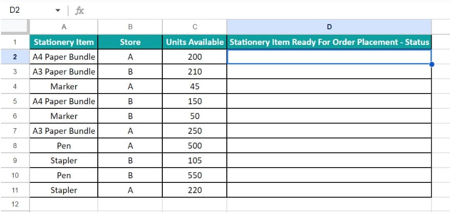
The requirement is to update the status of whether the stationery item is ready for order placement, provided the store is A, and the units available are equal to or exceed 200. Assume the target cell range is D2:D11.
Then, we can use the IF-AND advanced formula, similar to the IF-AND in Excel, in the target cells to secure the required outcome.
Step 1: Select cell D2 and enter the IF(), which has the same logic as the Excel IF function.

Next, enter the AND(), similar to the AND Excel function, as the IF() condition.
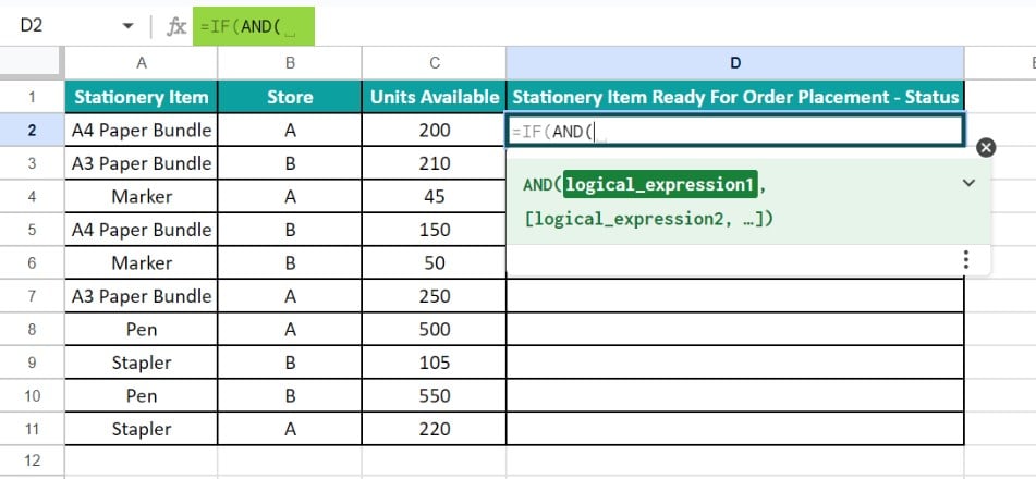
Step 2: Update the AND() argument values, followed by the IF() argument values, separated by commas, close the brackets, and press Enter.
=IF(AND(B2=”A”,C2>=200),”Stationery Item Ready For Order Placement”,”NA”)

Step 3: Utilize the fill handle to enter the IF-AND formula in the remaining target cells.
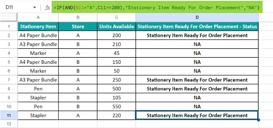
Let us see the cell D11 formula to understand its logic.
First the AND() checks whether the store mentioned in cell B11 is A and the units ordered value, specified in cell C11, is equal to or more than 200. Since both the conditions are true, the function returns the TRUE value as the required status.
#6 – IF OR Formula In Google Sheets
The IF-OR formula is an IF(), which uses the OR() in its condition to check multiple criteria in one go. The function output is the TRUE value when any one of the specified conditions is true. On the other hand, when all the conditions are false, the function output is the cited FALSE value.
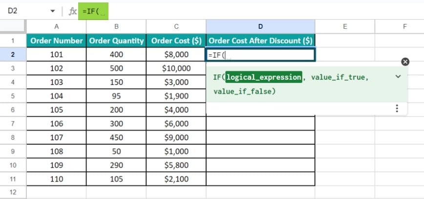
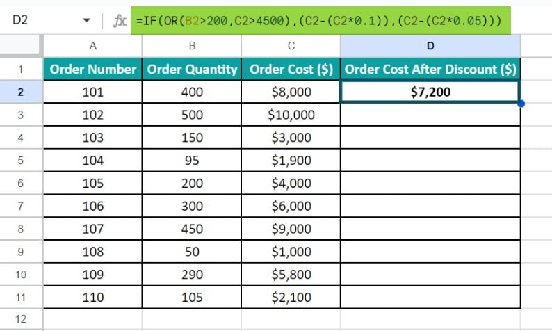
For example, we have a list of orders, their quantities and costs.

We must update the orders’ costs after the discount. However, the discount percentage will be 10% when the order quantity is more than 200, or the order cost exceeds $4,500. Otherwise, the discount percentage will be 5%. Assume that we must show the order costs after the discount in column D.
Then, here is how to apply the IF-OR advanced formula, in the target cells to acquire the required data.
Step 1: Choose cell D2 and enter the IF().
Next, enter the OR(), with the same logic as the Excel OR function, as the first argument value.
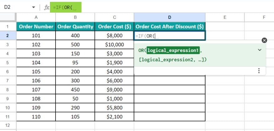
Step 2: Update the OR() argument values, followed by the IF() argument values, separated by commas. Next, close the brackets and press Enter.
=IF(OR(B2>200,C2>4500),(C2-(C2*0.1)),(C2-(C2*0.05)))
Step 3: Utilize the fill handle to implement the formula in the remaining target cells.

We shall check the cell D11 formula for the logic.
First, the OR() checks two conditions. It checks whether the order quantity in cell B11 exceeds the value of 200 and the order cost in cell C11 exceeds the value of $4,500. In this case, none of the conditions are true. So, the IF() condition is false, and the function returns the FALSE value.
The FALSE value in the IF() is an arithmetic expression. The formula multiplies the order cost value in cell C11 by 5% or 0.05, which is $105. Next, it deducts the product value of $105 from the order cost value in cell C11 to return $1,995 as the required order cost after the discount.
#7 – SUMIF Formula In Google Sheets
The SUMIF() is a formula that checks the specified condition in the cited range. It then adds the values in the corresponding rows, where the condition is true, of the range holding the potential values to add. However, the function can check only one condition to sum the values.
For instance, the source dataset lists teams and their date-wise customer calls attended data.

The task is to calculate the total customer calls the team FVD, cited in cell F1, attended. Assume we must display the determined sum value in cell F2.
Then, the steps to apply the SUMIF() in the target cell to secure the required result are as follows:
Step 1: Choose cell F2 and enter the SUMIF().

Step 2: Update the argument values, separated by commas. Next, close the brackets and press Enter.
=SUMIF(A2:A11,F1,C2:C11)

The SUMIF() accepts three input values. The first argument value is the range reference A2:A11, where the function must check the condition. Next, the second argument value is the reference to the cell F1 holding the required team’s name, FVD. Next, the third argument value is the range reference C2:C11, which contains the values we must add based on the cited condition.
So, the function checks for cells in the range A2:A11 where the team name is FVD. Cells A3, A9, and A10 meet the condition. So, the function adds the values in the corresponding rows 3, 9, and 10 of column C, which are the cells C3, C9, and C10 values. Thus, it returns the value of 840 as the required outcome.
#8 – CONCATENATE Formula In Google Sheets
The CONCATENATE formula in Google Sheets accepts text strings, and it appends them to return a single string as the output. The input values can be values, texts within double quotes, and cell references. On the other hand, if the strings to concatenate are in consecutive cells, we can supply the entire range as the input.
For example, the source dataset lists pharma companies and their revenues.
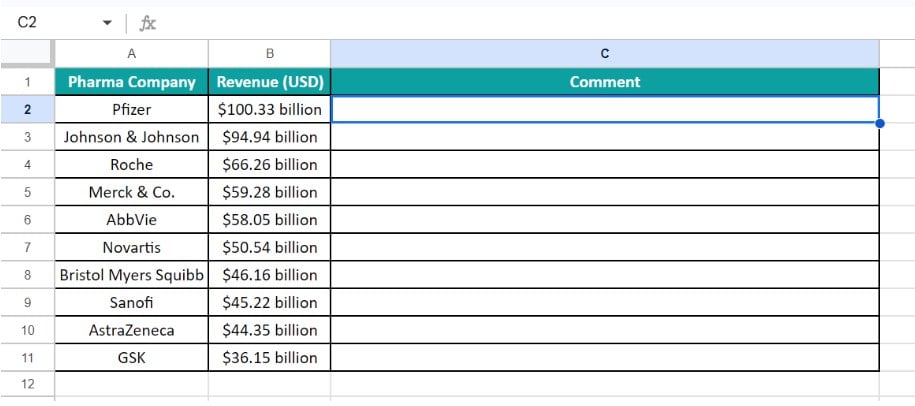
The task is to display the data as comments in column C using the CONCATENATE().
Step 1: Choose the target cell C2 and enter the CONCATENATE().
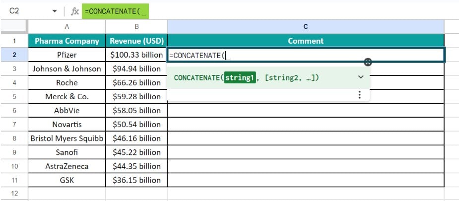
Step 2: Enter the argument values, separated by commas. Next, close the brackets and press Enter.
=CONCATENATE(“The revenue of the pharma company “,A2,” is “,B2,”.”)
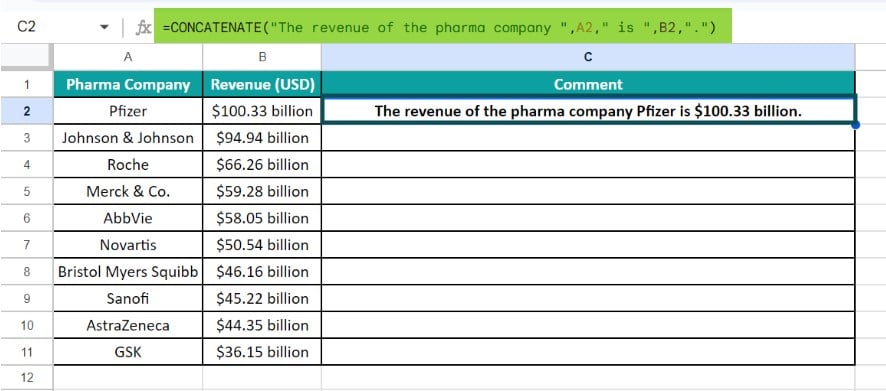
Step 3: Utilize the fill handle to implement the formula in the remaining target cells.
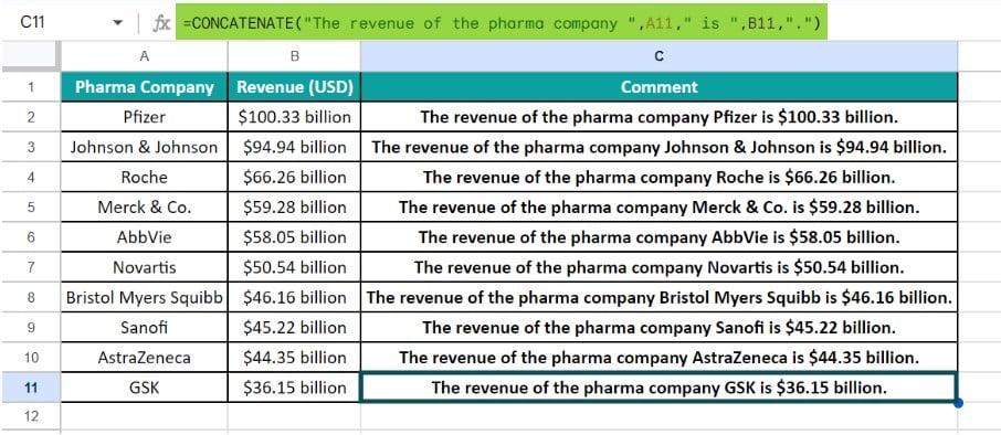
We shall check the cell C11 formula for the logic.
The CONCATENATE() accepts five input values. It appends the first text string, the cell A11 value, followed by another text, the cell B11 value, and one last string. So, the function returns one text string containing all the input texts and values as the required comment.
Please note that the function will not include spaces between the strings we want to append. We must enter the space characters when supplying the inputs to the function at the positions where we want them to appear in the concatenated string.
#9 – LEFT, MID, and RIGHT Formula In Google Sheets
The LEFT, MID, and RIGHT formulas return the section of the input string value, as indicated by the function names.
While the LEFT(), similar to the Excel LEFT function, determines the starting characters of the specified string, the MID(), like the Excel MID function, determines the middle characters. On the other hand, the RIGHT(), like the Excel RIGHT function, finds the ending characters of the specified string. Further, we must provide the number of characters to display while supplying the inputs to these functions.
For instance, we have a list of employees and their contact numbers.

Each contact number contains the country and area codes and the actual phone number.
The requirement is to extract the three components from the contact numbers and show them in the columns C:E cells.
Then, we can apply the LEFT(), MID(), and RIGHT() in columns C:E to achieve the desired outcome.
Step 1: Select the target cell C2 and enter the LEFT().

Step 2: Supply the argument values, separated by commas. Next, close the bracket and press Enter.
=LEFT(B2,1)

The LEFT() accepts two input values. While the first argument value is the reference to cell B2, containing the contact number, the second is the value of 1, which is the number of characters we must show in the output.
So, the function shows the first character in the contact number from the left as the required country code, which is the value of 1.
Step 3: Choose cell D2 and enter the MID().

Step 4: Supply the argument values, separated by commas. Next, close the bracket and press Enter.
=MID(B2,3,3)

The MID() accepts three inputs. The first argument value is the reference to the cell B2 containing the contact number. Next, the second argument value of 3 indicates the position from the left of the contact number, from where we must start counting the middle characters we wish to display as the output. Next, the third argument value of 3 indicates the number of characters we must count from the specified starting point to display as the middle characters.
Thus, the function counts three characters from the third character in the contact number, which is 847, to return it as the required area code.
Step 5: Select cell E2 and enter the RIGHT().

Step 6: Supply the argument values, separated by commas. Next, close the bracket and press Enter.
=RIGHT(B2,8)

The RIGHT() accepts two input values. While the first argument value is the reference to cell B2, containing the contact number, the second is the value of 8, which is the number of characters we must show in the output.
So, the function shows the last eight characters in the contact number from the right as the required phone number, which is the value of 437-8315.
Step 7: Choose the range C2:E2, and using the fill handle, feed the formulas in the remaining target cells.

#10 – OFFSET Formula In Google Sheets
The OFFSET formula in Google Sheets determines a reference to a cell range that is a cited number of rows and columns from a cell or cell range. The reference that is obtained can be a cell or a cell range. We can cite the count of rows and columns to be determined.
For example, the source dataset lists the monthly expenses and savings.
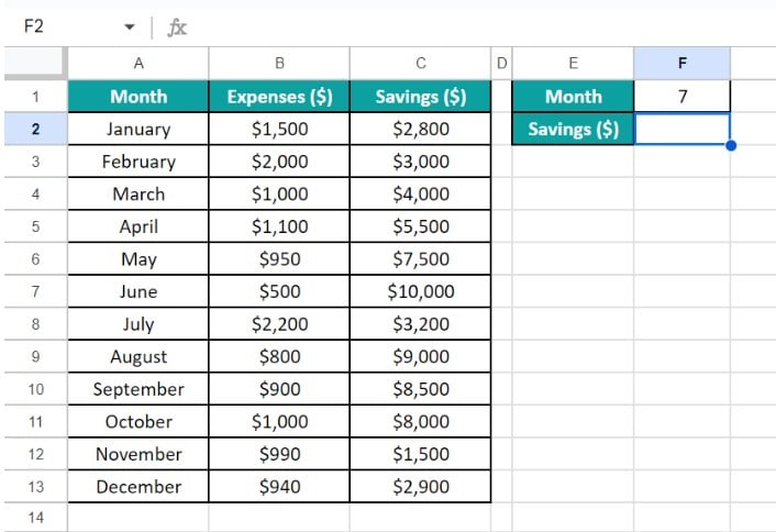
We must determine the savings made in the seventh month, July, as cited in cell F1. We shall take cell F2 as the target cell.
Then, we can apply the OFFSET(), similar to the Excel OFFSET function, in the target cell to fetch the required data.
Step 1: Select cell F2 and enter the OFFSET().

Step 2: Supply the argument values, separated by commas. Next, close the bracket and press Enter.
=OFFSET(A1,F1,2)

The OFFSET() accepts three input values. The first argument value is the reference to cell A1, from where we must count the specified number of rows and columns. Next, the second argument value is the reference to cell F1 holding the number of rows we must count from cell A1. Next, the third argument value of 2 indicates the number of columns we must count from cell A1.
Thus, the function counts seven rows and two columns from cell A1, which is row 8 and column C. It then returns the value in the cell where row 8 and column C meet, which is the cell C8 value of $3,200, as the required savings value.
Frequently Asked Questions (FAQs)
We can use the INDEX MATCH advanced formula in Google Sheets, as explained below with an illustration.
The source dataset contains date-wise storage container dispatch status and inventory-level data.
We need to update the dispatch status for the storage container specified in cell G1 and showcase the output in cell G2.
We could have used the VLOOKUP() in the target cell. However, the search range is on the right of the return value range, which leads to the function returning an error value.
Instead, we can apply the INDEX-MATCH advanced formula in the target cell to secure the required status.
Step 1: Choose cell G2, enter the INDEX-MATCH formula, and press Enter.
=INDEX(A2:D11,MATCH(G1,C2:C11,0),2)
First, the MATCH() searches for the lookup value of RTT_256, cited in cell G1, for an exact match in the lookup range C2:C11. It finds the exact match in cell C7. So, the function returns the value of 6 since the lookup range starts from row 2 of the sheet.
Next, the INDEX() returns the value in the cell where row 7 of the sheet, which is actually row 6 in the reference range, and the second column of the reference range, column B, meet. Thus, the function output is the cell B7 value, Storage Container Dispatched.
The advanced Google Sheets formulas are the same as Excel, except some inbuilt functions may show the argument value names in their syntaxes different from those in Excel.
However, their functionalities remain the same.
The difference between XLOOKUP and VLOOKUP advanced formulas in Google Sheets are as follows:
• Unlike the VLOOKUP(),the XLOOKUP() does not have the limitation of looking up the search key value in the first column of the lookup range.
• The XLOOKUP() includes an argument value to specify the text when a match is not found, which is not available in the VLOOKUP().
Download Template
This article must be helpful to understand the Advanced Google Sheets Formulas, with its formula and examples. You can download the template here to use it instantly.
Recommended Articles
This has been a guide to What Is Advanced Google Sheets Formulas. We explain the list of top 10 advanced formulas in Google Sheets with examples. You can learn more from the following articles –

Leave a Reply