
OFFSET Function Definition
OFFSET is a lookup and reference function in Excel that returns a reference to a cell or range of cells, or in other words, a specified number of rows and columns from a specified cell or range of cells.
For the OFFSET function, we need to enter the starting cell address. Then we need to enter the number of rows to move down or the up, the number of columns to move left or right, and then we need to mention the number of rows and columns to offset from the starting position of the cell provided. For instance, we have the following monthly sales data in an Excel spreadsheet.
Use this OFFSET Function In Excel Template to follow along with the examples in this article.
Download Excel Template
If we want to get the value of cell B6 from the starting cell A1, you can enter the below formula in cell E1.
=OFFSET(A1,5,1)

Starting from cell A1 OFFSET function moves 5 rows down and then moves 1 column to the right. Finally, it locates cell B6 and returns the value from cell B6. So we can restructure the formula like the following to understand it better.
=OFFSET(A1,5 Rows Down,1 Column to Right)
Like this, the OFFSET function will be used to offset cells based on the starting cell provided.
Key Takeaways
- The OFFSET function returns the reference from the starting position of the cell or range of cells and is based on the specified number of rows and columns.
- It is used to create dynamic ranges, dynamic drop-down lists, and dynamic sum formulas for pivot tables and charts.
- Using the OFFSET function, one can look up values from left to right and vice versa. So, it can be used as an alternative to the VLOOKUP function.
- We can use OFFSET function in Excel as a dynamic range for SUM, AVERAGE, and other aggregative functions.
OFFSET Excel Formula
Below is the syntax of the OFFSET formula in Excel:

The OFFSET function has three mandatory arguments and two optional arguments:
- Reference: This is the reference of the cell or range of cells from where you need to start the offset. Thus, it is the starting point of the offset and is a mandatory argument.
- Rows: The number of rows to move up or down from the starting point. If you mention a positive number, it will move down from the starting position, and if you mention a negative number, it will move up from the starting position. It is a mandatory argument.
- Cols: The number of columns to move to the right or left from the starting point. If you mention a positive number, it will move to the right from the starting position, and if you mention a negative number, it will move to the left from the starting position. It is a mandatory argument.
- [height]: The number of rows we need to return in the returned reference. It is an optional argument.
- [width]: The number of columns we need to return in the returned reference. It is an optional argument.
How To Use OFFSET Function?
Let us look at a basic Offset function in Excel example.
For instance, we have an Excel spreadsheet containing employee salary details.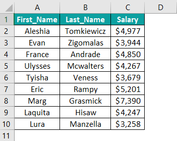
Assume we need to get the reference of cell C8 starting from cell A1. We can achieve this in the following steps using OFFSET function.
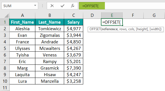
- Enter the OFFSET function in cell E1.

- The reference cell is the starting position where we need to start the offset. In this case, it will be from cell A1.
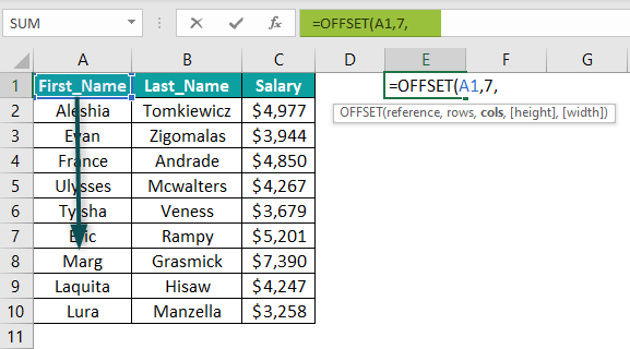
- We need to locate cell C8, so the number of rows to move down here is 7. Enter 7 for rows argument.

- After moving down 7 cells to the down, we reference cell A8. We need to move 2 columns to the right from this cell to reach C8. Enter C8 for the cols argument.

Since we are trying to locate a single cell reference, ignore the last two arguments. Close the bracket and hit the Enter key to get the result.
The OFFSET function returned the reference of cell C8, i.e., $7,390.
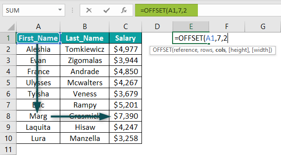

The OFFSET function started the offset from cell A1, moved 7 cells down, moved 2 columns to the right, and offset cell C8.
Examples
Let us look at some advanced offset function in Excel examples to understand its working:
Example #1: Get the Sum Using the OFFSET Function
We have the monthly-wise city sales in an Excel spreadsheet.

We will create a dynamic formula that gives us the total sales for the desired month.
Step 1: Create a month, and total sales targeted cells in column G like the following.

Step 2: Create a month number drop-down in cell H1 like the following.

Step 3: In cell H2, enter the OFFSET function.

Step 4: Select the reference cell as cell A1.

Step 5: Starting from cell A1, the number of rows we need to move down depends on the month number we select in cell H1 from the drop-down list. Hence, the rows argument will be an H1 cell reference.

Step 6: After moving several rows down, we need to move 1 column to the right. Enter 1 for cols argument.

Step 7: Since we are looking at one month of total sales at a time, the height will be 1.

Step 8: The width will be the number of cities in our data table. So, this will be 4.

Step 9: This ends the OFFSET function. Close the bracket and hit the Enter key.

Step 10: Select the month number in cell H1 from the drop-down.

Step 11: Since we have selected the month number as 4, the OFFSET function moves down 4 cells from cell A1 and takes the reference of the month Apr in cell A5. The OFFSET function moves 1 to the right and offsets 1 row and 4 columns from this cell reference.
This is why we get all the values from the given height and width. To get the sum of these cells, we need to wrap the OFFSET function with the SUM function.

Now the combination of the SUM and OFFSET functions gives the given month number’s total sales.
Change the month number in cells H1 and H2 (SUM and OFFSET functions) returns the total sales for the given month.

Example #2: Dynamic Drop-Down List by Using OFFSET Function
Creating a drop-down list is common but making it dynamic requires advanced formulas. The OFFSET function provides an opportunity to create a dynamic drop-down.
For instance, we have the following drop-down list for month names in an Excel spreadsheet.

The issue with this drop-down is an addition to the month list will not reflect in the drop-down.
We have added the month name Jun in cell A7, but the drop-down list does not show it.

However, using the OFFSET function, we can create a dynamic drop-down.
Step 1: Go to the Data tab and click on the Data Validation option.

Step 2: This opens the data validation window.

Step 3: Here, it is taking the reference of cells A2:A6. So, any changes after cell A6 are not affecting the drop-down list. So, enter the below formula in the Source box.
=OFFSET(A2,0,0,COUNTA(A2:A100),1)

Click on OK. The values entered in cells A2:A100 are updated in the drop-down list.

Formula Explanation:
=OFFSET(A2,0,0,COUNTA(A2:A100),1)
=OFFSET(A2: The OFFSET function starts the offset from cell A1.
=OFFSET(A2,0,0: It moves down 0 rows and 0 columns.
=OFFSET(A2,0,0,COUNTA(A2:A100),: COUNTA function will return the number of rows we have data in cell A2:A100, and then the OFFSET function offsets the same number of rows starting from cell A2.
=OFFSET(A2,0,0,COUNTA(A2:A100),1): Since only one column we are offsetting, the last argument will be 1.
Like this, we can create a dynamic drop-down list by using the OFFSET function.
Note: We’ve chosen the range of cells A2:A100 to enter the values and reflect them in the drop-down, so we can keep going until we come to cell A100. You can also mention it as A10 (9 months in this example) or A13 (to enter 12 months of a year).
Example #3: OFFSET As an Alternative To VLOOKUP
VLOOKUP function is designed to lookup values from left to right only. Hence, whenever the data structure is right to leave, VLOOKUP cannot fetch the value.
For instance, look at the following image.

In the above table, months are at the extreme left of the result column “Sales,” so VLOOKUP works without any problem.
However, when the Month column is shifted next to the Sales column, VLOOKUP will not work.

We often use a combination of INDEX and MATCH functions for this kind of data structure. However, we can also use OFFSET, MATCH, and ROWS functions.
Enter the below formula to get the result.
=OFFSET(A2:B6,MATCH(D2,OFFSET(A2:B6,0,1,ROWS(A2:B6),1),0)-1,0,1,1)

The formula looks complicated but works fine here, and the result we have in cell E2 is the sales for the month Mar, i.e., $3,389.
The OFFSET function offsets the range A2:B6, and the MATCH function returns the row number for the desired month name in cell D2 with the help of another OFFSET function and ROWS function.
Important Things To Note
- OFFSET function returns the #REF error if the row and column numbers are wrong.
- It always recalculates the values whenever there is a change in the source data and keeps the Excel busy for longer. Hence, it is suggested not to use too many OFFSET functions.
- The OFFSET function is often difficult to review whenever nested OFFSET is used to make the reference dynamic.
- The alternatives to the OFFSET function are INDEX Function, INDIRECT Function, and Excel Tables.
Frequently Asked Questions (FAQs)
The OFFSET function is a lookup and reference function in Excel. OFFSET function in Excel returns a reference to a cell or range of cells offset from the desired cell by a specified number of rows and columns.
Let us look at the data of Sales Territory Regions.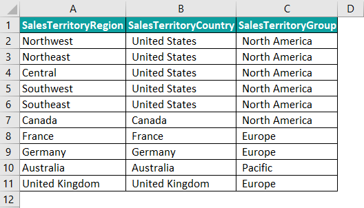
Assuming we need to get the reference of cell A3 from cell C6, we can enter the following formula in the desired cell.
=OFFSET(C6,-3,-2)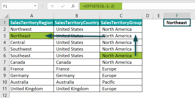
The OFFSET function starts the offset from cell C6, moves 3 rows to the top, then moves 2 columns to the left and locates cell A3.
The OFFSET function creates a dynamic drop-down list and dynamic sum formula, especially for pivot tables and charts.
If your OFFSET function is not working, it is mainly because of the REF# issue. For instance, look at the following image.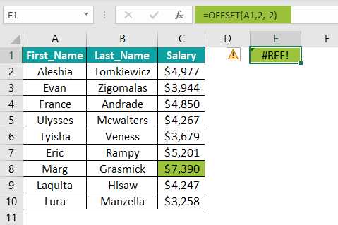
In the above image, the OFFSET function starts the offset from cell B8, moving 2 cells down but 2 to the left. This is because offset starts from cell B8, and can only move one column to the left. Since it cannot move two columns to the left, the OFFSET function returns the #REF error.
Use this OFFSET Function In Excel Template to follow along with the examples in this article.
Download Excel Template