Advanced Excel Formulas

List Of Top 10 Advanced Excel Formulas

We will understand the following Top 10 Advanced Excel Formulas with examples.

1. VLOOKUP Formula in Excel.
2. XLOOKUP Formula in Excel.
3. INDEX Formula in Excel.
4. MATCH Formula in Excel.
5. IF AND Formula in Excel.
6. IF OR Formula in Excel.
7. SUMIF Formula in Excel.
8. CONCATENATE Formula in Excel.
9. LEFT, MID, and RIGHT Formula in Excel.
10. OFFSET Formula in Excel

#1 – VLOOKUP Formula in Excel

VLOOKUP, or the Vertical Lookup function, retrieves the values from the dataset based on the given lookup_value. It looks up the values from left to right from the lookup_value column.

The syntax of the VLOOKUP function is,

The arguments of the VLOOKUP function are,

• lookup_value: The value for which we are trying to retrieve the result from the table_array (2^nd argument). It is a mandatory argument.
• table_array: It will be either range or table_array where we search for the lookup_value. It is a mandatory argument.
• col_index_num: In a given table_array, the column we are looking for the result. It is a mandatory argument.
• [range_lookup]: In this optional argument, we need to specify the kind of match we need:
  • 0 or FALSE – It will search for the exact match of the lookup_value in the table_array. If nothing is specified, 1 or TRUE will be the default mode.
  • 1 or TRUE – It will search for the approximate match of the lookup_value in the table_array.

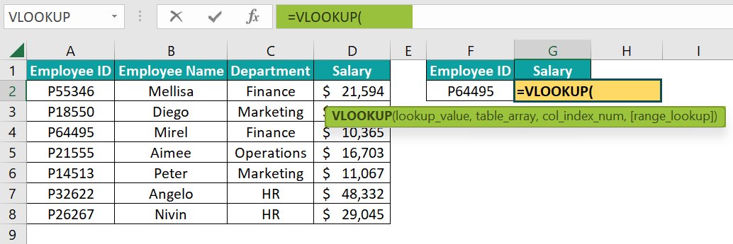
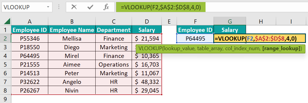
For instance, we have the following employee data in an Excel spreadsheet. We will find the salary of the employee with the employee id “P64495”.

The steps to find the salary of the P64495 employee using the VLOOKUP formula are,

• Step 1: Select cell G2, and enter the formula =VLOOKUP(

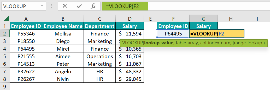
• Step 2: For the lookup_value select employee id cell F2. The formula now is =VLOOKUP(F2

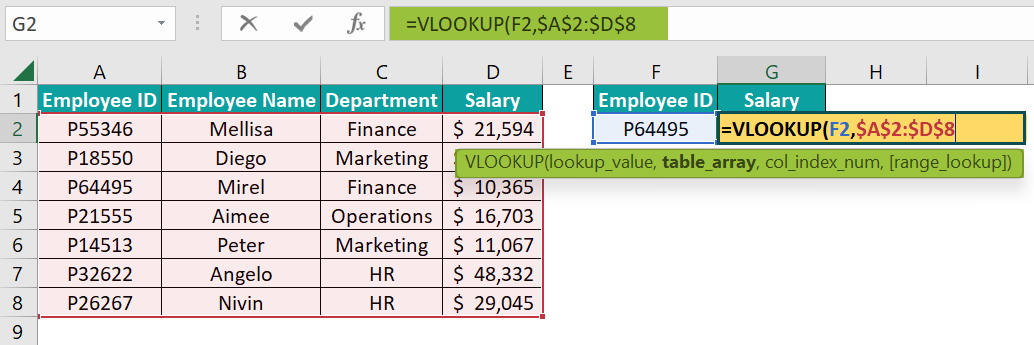
• Step 3: For the table_array, select the employee table, A1:D8, and make it an absolute reference by pressing the F4 key because when we use the same formula for multiple employee ids, table_array should remain the same. The formula now is =VLOOKUP(F2,$A$2:$D$8

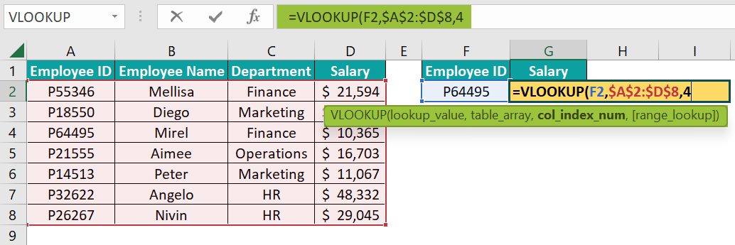
• Step 4: Next, from the selected table_array, we need the salary column, and that column number is 4. Now, the formula is =VLOOKUP(F2,$A$2:$D$8,4

• Step 5: Finally, since it will be an exact match, enter either FALSE or 0, and close the brackets. The complete formula is =VLOOKUP(F2,$A$2:$D$8,4,0)

• Step 6: Press the “Enter” key to get the result.

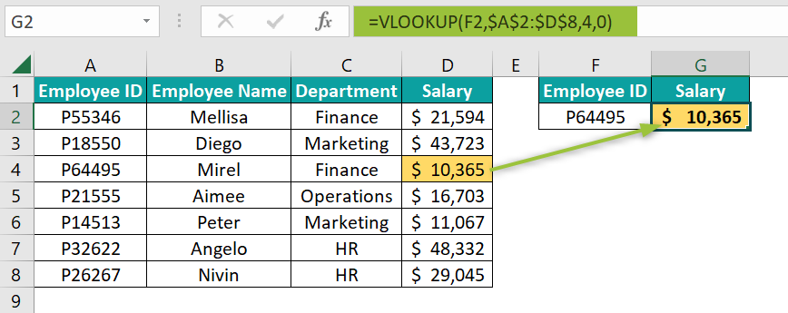
Output Observation: The VLOOKUP function goes through the range of cells from A2:D8 and looks for the employee id “P64495” and returns the value from the 4^th column, and the salary of the employee is $10,365.

#2 – XLOOKUP Formula in Excel

XLOOKUP is the newly added feature with the Office 365 version of Excel. It is the advanced and versatile version of all the other lookup functions like VLOOKUP, HLOOKUP, INDEX and MATCH, and LOOKUP.

XLOOKUP allows the user to fetch the desired value from the data table. The data table structure is not a concern here because it can retrieve the values from left to the right, right to left, top to bottom, and vice versa.

The syntax of the XLOOKUP function is a bit more complex than other lookup functions but versatile and flexible and is as follows,

The arguments of the XLOOKUP function are,

• lookup_value: Thevalue for which we try to retrieve the result from the return array (3^rd argument). It is a mandatory argument.
• lookup_array: It will be either range or table_array where we search for the lookup_value. It is a mandatory argument.
• return_array: It is the array from which we need to get the desired result for the lookup_value provided in the first argument. It is a mandatory argument.
• [if_not_found]: If the lookup_value is not available in the lookup_array we end up getting a #N/A error. However, we can get an alternative result instead of the default #N/A error by providing an alternative result here. It is an optional argument.
• [match_type]: In this argument, we need to specify the kind of match we need to do:
  • 0 – Exact Match, this will search for the exact match of the lookup_value in the lookup_array. If nothing is specified 0, will be the default mode.
  • -1 – It will again look for an exact match, but if not found, it will look for the next smaller item than the lookup_value.
  • 1 – It looks for an exact match, but if not found, it will look for the next larger item than the lookup_value.
  • 2 – It performs partial lookup operations using wildcard characters like an asterisk (*) and tilt (~).
  • [search_mode]: In this argument, we need to specify how XLOOKUP searches for the lookup_value.
  • 1 – It is the default searching option. It will allow the XLOOKUP to start searching from top to bottom in the lookup_array.
  • -1 – It will do the searching from down to top. It is helpful if we want to find the last matching result for the lookup_value.
  • 2 – It will help us to do binary searching, and data needs to be sorted in ascending order. If not sorted, we will get either the wrong result or an error.
  • 2 – It will help us to do binary searching, and data needs to be sorted in descending order. If not sorted, we will get either the wrong result or an error.

Let us continue with the same example of VLOOKUP, and we have modified the data structure, and then applied the XLOOKUP function.

Here, we have the salary information (in column B) before the employee id column (in column C). In this data structure, VLOOKUP cannot be applied because the lookup_value column “Employee ID” is to the right of the result column “Salary”. VLOOKUP can fetch the values from the columns that are to the right of the lookup_value column. However, XLOOKUP does not have these limitations.

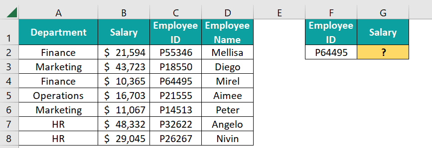
The steps to find the salary of the P64495 employee using the XLOOKUP formula are,

• Step 1: Select cell G2, and enter the formula =XLOOKUP(

• Step 2: For the lookup_value select employee id cell F2. The formula now is =XLOOKUP(F2,

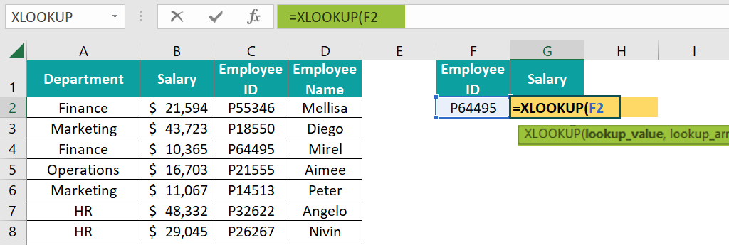
• Step 3: For the lookup_array, select the employee table, C2:C8, and make it an absolute reference by pressing the F4 key because when we use the same formula for multiple employee ids, table_array should remain the same. The formula now is =XLOOKUP(F2,$C$2:$C$8,

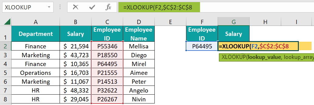
• Step 4: For the return_array argument, we need to choose from which column we need the result, i.e., the salary column from B2:B8, and close the brackets. The complete formula is =XLOOKUP(F2,$C$2:$C$8,$B$2:$B$8)

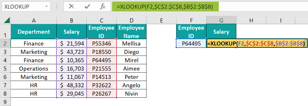
[Note: The XLOOKUP function does not require other parameters like “Match Mode” to be specified here because, by default, it searches for the exact match, i.e., 0 or FALSE.]

• Step 5: Press the “Enter” key to get the result.

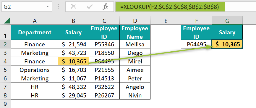
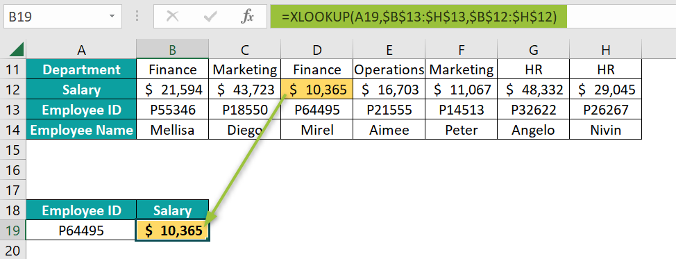
Output Observation: The result is the same as the VLOOKUP but what matters here is the data structure. To understand the versatility of the XLOOKUP function, let us convert the data structure from vertical to horizontal.

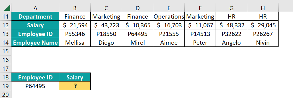
Whenever the data structure is horizontal, we use the HLOOKUP function, but XLOOKUP can retrieve the values from both horizontal and vertical data structures.

Apply the XLOOKUP as we have applied in the above example, and it gives the same result.

#3 – INDEX Formula in Excel

INDEX Excel function enables users to fetch the value from the desired column or row depending on the requirement. It retrieves the value from a single cell, entire column, or entire row values.

The syntax of the INDEX function comes in two forms, i.e., Array & Reference.

The arguments of the INDEX function [array & reference] are,

• array: The range of a cell (row or column) or an array constant. It is a mandatory argument.
• reference: The cell range or references. It is a mandatory argument.
• row_num: From the first argument Array, which row number to fetch the value. It is a mandatory argument.
• [column_num]: It is an optional argument. When we need to fetch the value from a specified row and specified column, we will use it.
• [area_num]: It is an optional argument. It is used in rare-case scenarios. When we supply multiple ranges for an argument by providing the area number, we can select the reference from all the available ranges.

For instance, we will use the same data from the above examples. We will retrieve the salary information for the employee id “P64495” using the INDEX function.

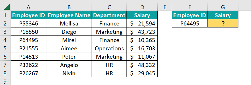
The steps to find the salary of the P64495 employee using the INDEX formula are,

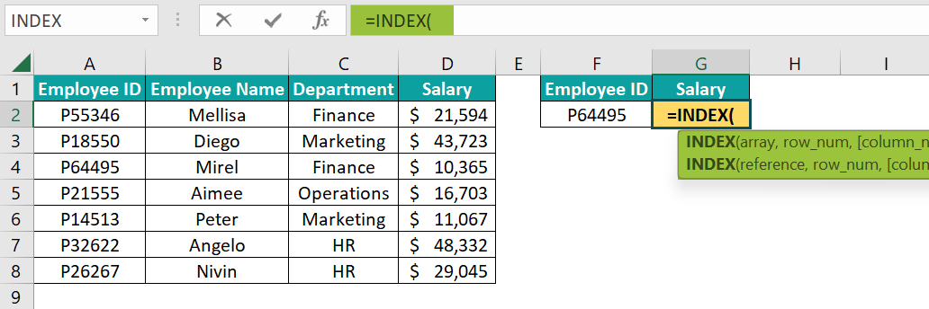
• Step 1: Select cell G2, and enter the formula =INDEX(

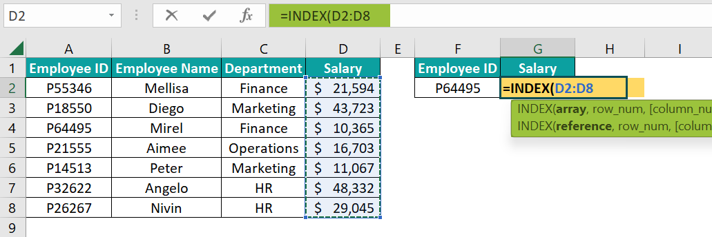
• Step 2: For the array argument, we must choose the result column, i.e., the salary column.

• Step 3: Next, we need to mention the row number of the employee id that we are looking for. For employee id “P64495”, the row number is 3.

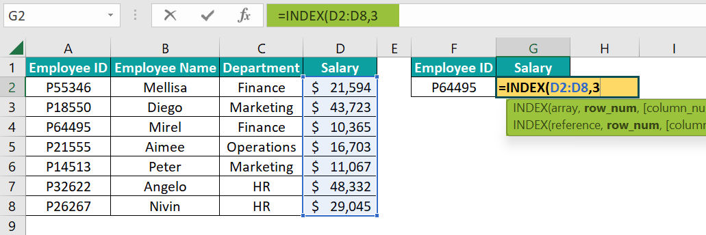
• Step 4: Since we are using one-way lookup, we can ignore the column number argument. Close the bracket and press “Enter”. The complete formula is =INDEX(D2:D8,3)

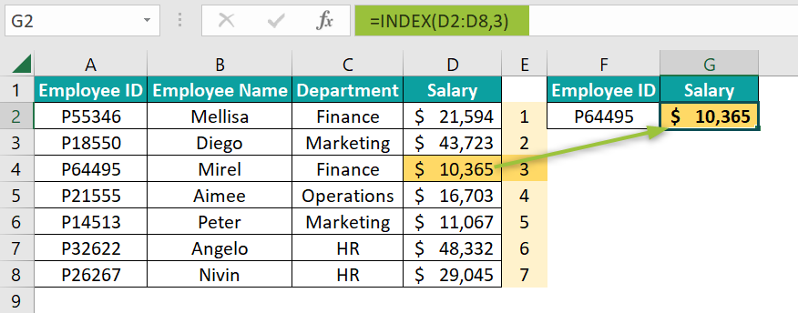
The result looks fine. However, entering the row number based on the employee id is not the best practice because whenever the employee id changes, the result, too, should change dynamically.

To make the row number dynamic, we should combine the INDEX function & the MATCH function.

Enter the MATCH function for the row number argument of the INDEX function, .

For the lookup_value of the MATCH function, chooses the employee id cell F2.

We must choose the employee id column in the data table from A2:A8, for the lookup_array,

For the match, type choose the exact match, i.e., 0.

Close the brackets to both the INDEX and MATCH functions and press “Enter” to get the result. The complete formula is =INDEX(D2:D8,MATCH(F2,A2:A8,0))

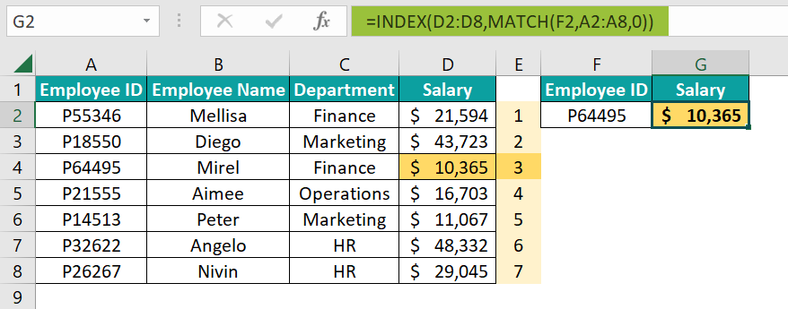
Here the MATCH function dynamically returns the row number for the given employee id, and then the INDEX function will return the result from the row number given by the MATCH function.

#4 – MATCH Formula in Excel

The MATCH excel function retrieves the cell address of the desired value from the given table_array. The MATCH function is often used as a supporting function for the INDEX and VLOOKUP formulas to fetch the values dynamically.

The syntax of the MATCH function is,

The arguments of the MATCH function are,

• lookup_value: The value whose position we want to locate in the lookup_array (second argument). It is a mandatory argument.
• lookup_array: It will be either range or table_array where we search for the lookup_value. It is a mandatory argument.
• [match_type]: It is an optional argument. It is the matching criteria that we need to define for the lookup_value. It can be:
• 1 = It will look for the largest value, either less than or equal to the lookup_value we have provided, and return the approximate match. It requires lookup_array to be arranged in ascending order (lower to higher or A to Z).
• 0 = It will check and return the exact match to the lookup_value, irrespective of how the data is arranged or sorted.
• -1 = It will search for the smallest value, which is either greater than or equal to the lookup_value we have provided, and return the approximate match. It requires the lookup_array to be arranged in descending order (higher to lower or Z to A).

For instance, we will use the same data from the above examples.

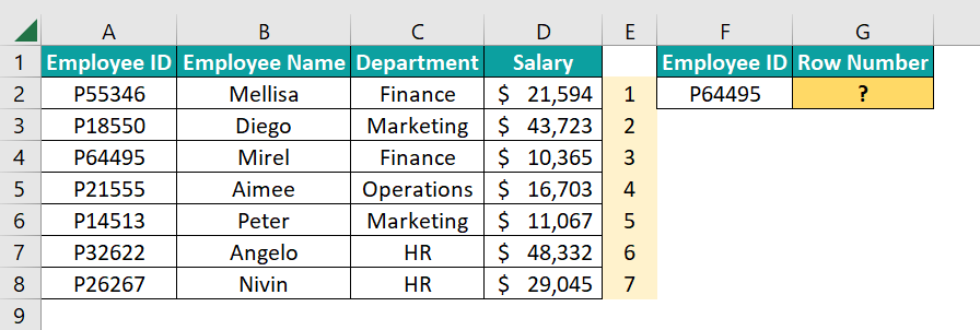
The steps to find the salary of the P64495 employee using the XLOOKUP formula are,

• Step 1: Select cell G2, and enter the formula =MATCH(

• Step 2: The lookup_value will be the employee id and provide the cell reference as F2.

• Step 3: The lookup_array will be the employee id list, so select the range of cells A2:A8.

• Step 4: At last, provide the matching type as 0 – Exact Match.

• Step 5: Close the bracket and press “Enter” to get the result. The complete formula is =MATCH(F2,A2:A8,0)

The position of the employee id “P64495” in the range A2:A7 is 3.

The real usage of the MATCH function is when used with VLOOKUP and INDEX functions.

For instance, we must fetch the Employee Name, Department, and Salary information based on the Employee ID.

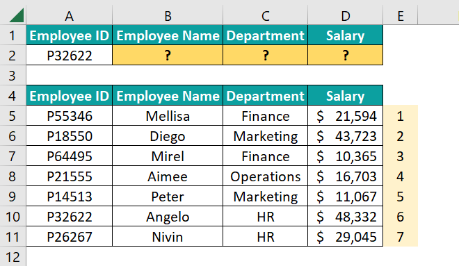
Let us apply the VLOOKUP function to fetch the Employee Name.

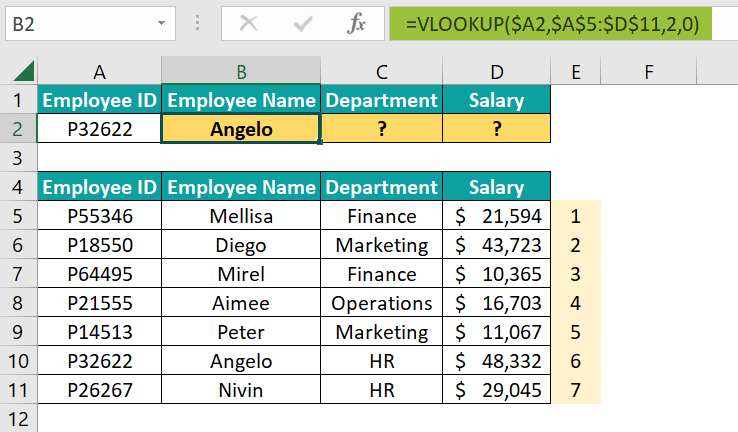
To fetch the employee’s name, we have mentioned the column INDEX number as 2. Similarly, to fetch the department and salary information, we need to mention the column INDEX numbers as 3 and 4, respectively. However, using the MATCH function, we can dynamically retrieve the column numbers based on the column headers. The complete formula is =VLOOKUP($A2,$A$5:$D$11,MATCH(B1,$A$4:$D$4,0),0)

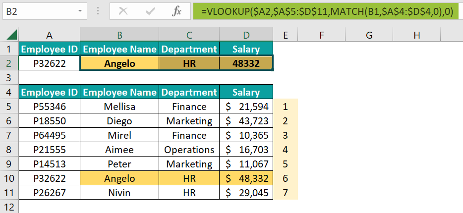
Now column number will be retrieved dynamically by using the MATCH function. The MATCH function looks for the respective headers in the range A4:D4 and returns the column number of the respective header. Then, based on the column number provided by the MATCH function, the VLOOKUP function retrieves the value from that column number.

#5 – IF AND Formula in Excel

IF and AND are logical functions in Excel. We can apply logical_tests and arrive at results based on the TRUE or FALSE nature of the IF function.

The syntax of the IF function is:

The arguments of the IF Excel function are:

• logical_test: The logical_test that we need to apply to evaluate the result. It is a mandatory argument.
• [value_if_true]: If theapplied logical_test is TRUE, then what is the value needed to return. It is an optional argument.
• [value_if_false]: If theapplied logical_test is FALSE, then what is the value needed to return. It is an optional argument.

With the AND Excel function, we can apply logical_test and if all the applied logical_test are correct, then it will return TRUE, and if any one of the logical_test is not correct, it will return FALSE.

The syntax of the AND function is:

The arguments of the AND function are:

• logical 1: It is the first logical_test to apply. It is a mandatory argument.
• [logical 2]: It is the second logical_test to apply. It is an optional argument.

For example, let us apply the IF and the AND functions together for the following data in Excel.

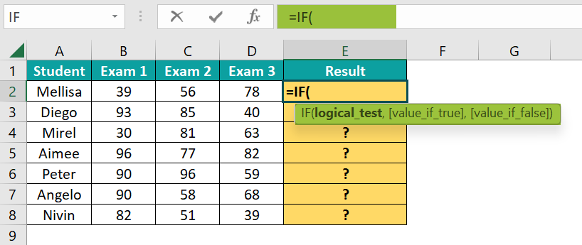
We have students and 3 different exam scores. To get the result, we are using the parameter as follows.

• If all the exam scores are greater than 50, then we need the result as “Shortlisted” and if any one of the exam scores is less than 50, we need the result as “Not Shortlisted”.

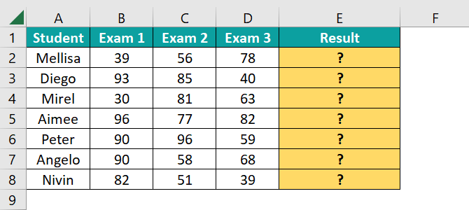
The steps to get the required results using the IF & AND formulas are,

• Step 1: Select cell E2, and enter the formula =IF(

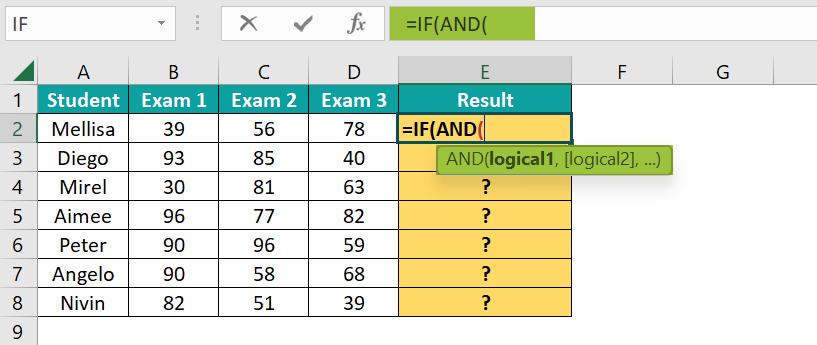
• Step 2: The logical_test that we need to apply here is to check whether all the 3 exam scores are >50 or not. Since we need to apply 3 logical_test and those tests should be correct to arrive at one result, so enter AND function inside the IF conditions. So the formula is =IF(AND(

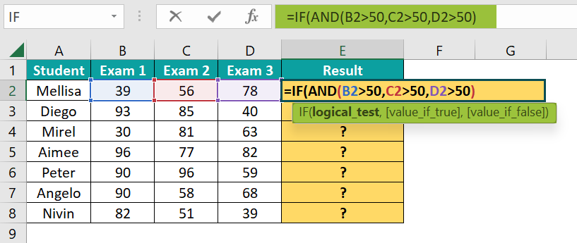
• Step 3: Apply logical_tests for all three exams as shown below. Three exams in cells B2, C2, and D2 have been applied to the logical_test to check whether the score is >50 or not.

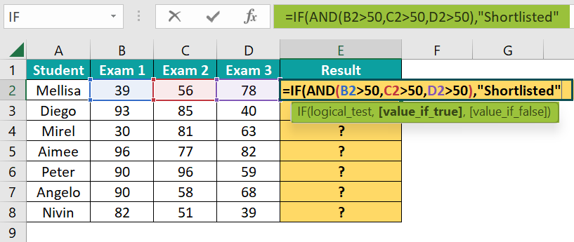
• Step 4: If all the test scores are >50, then AND function will return TRUE. If the logical_test result is TRUE, then we need the result as “Shortlisted”, so enter this value for the [value_if_true] parameter.

• Step 5: If the logical_test result is FALSE, then we need the result as “Not Shortlisted”.

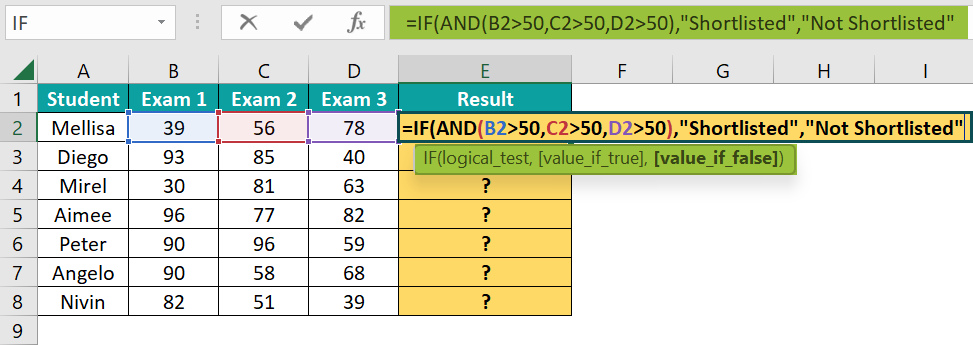
• Step 6: Close the bracket and press “Enter” to get the result. The complete formula is =IF(AND(B2>50,C2>50,D2>50),”Shortlisted”,”Not Shortlisted”)

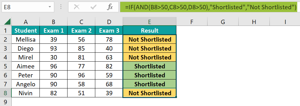
If we look at the first result in cell E2, we have the result as “Not Shortlisted” because not all the exam scores are >50. In Exam 1 score is <50, and even though the other 2 exam scores are >50, the eventual result is FALSE in AND function.

#6 – IF OR Formula in Excel

With the OR excel function, we can apply logical_tests, and if any one of the logical_tests is correct, then OR() will return the eventual result as TRUE. Also, OR() will return FALSE only if all the logical_tests are incorrect.

The syntax of the OR function, the same as the AND function, is,

Let us use the same data from the above example with a slight change in numbers. This time we will modify the logical_test as “If any of the exam scores is >50, then the result will be “Shortlisted”, and if none of the exam scores are >50, then the result will be “Not Shortlisted”.

Apply the logical_test like the one we have applied earlier but this time with the OR function.

The complete formula is =IF(OR(B2>50,C2>50,D2>50),”Shortlisted”,”Not Shortlisted”)

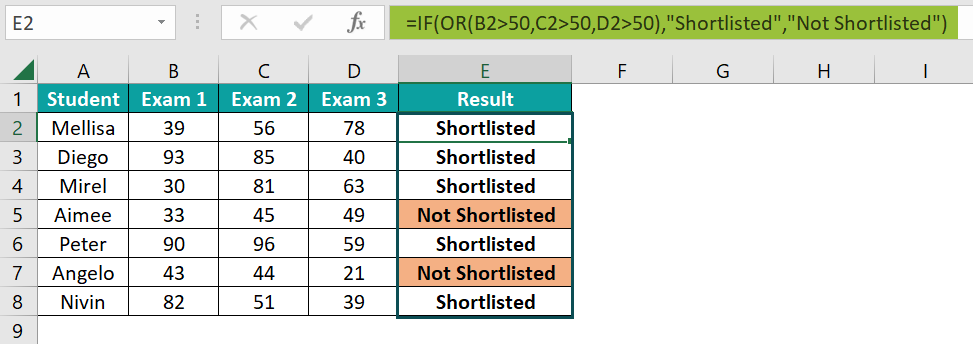
Look at the first result. The exam 1 score is not >50, but the other exam 2 scores are >50, so the result is “Shortlisted”. Similarly, look at the colored rows (5 & 7). All the exam scores are <50, so the result is “Not Shortlisted”.

#7 – SUMIF Formula in Excel

The SUMIF excel function is used to add the values based on the set of criteria given. The function can accept only one criteria.

The syntax of the SUMIF function is,

The arguments of the SUMIF function are,

• range: The cell range we will apply the criteria. It is a mandatory argument.
• criteria: In the given range, the cells that need to be considered for calculation. It is a mandatory argument.
• [sum_range]: The column to be summed based on the criteria given. It is an optional argument.

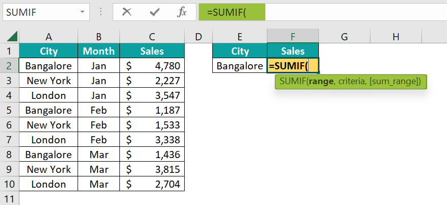
For instance, we have the following city-wise sales in Excel.

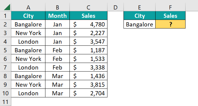
The steps to calculate the sum of sales only for the “Bangalore” city using SUMIF() are,

• Step 1: Select cell F2, and enter the formula =SUMIF(

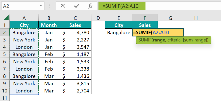
• Step 2: Select the range as a city column from A2:A10.

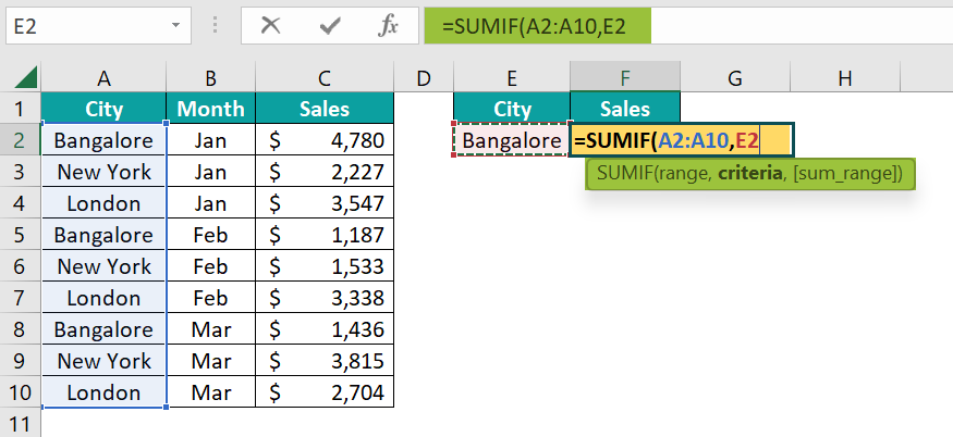
• Step 3: From the selected range, the criteria to apply is “Bangalore”, so choose cell reference E2.

• Step 4: The sum range will be the sales column from C2:C10.

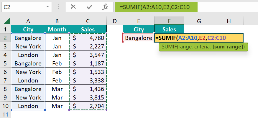
• Step 5: Close the bracket and press “Enter”. The complete formula is =SUMIF(A2:A10,E2,C2:C10)

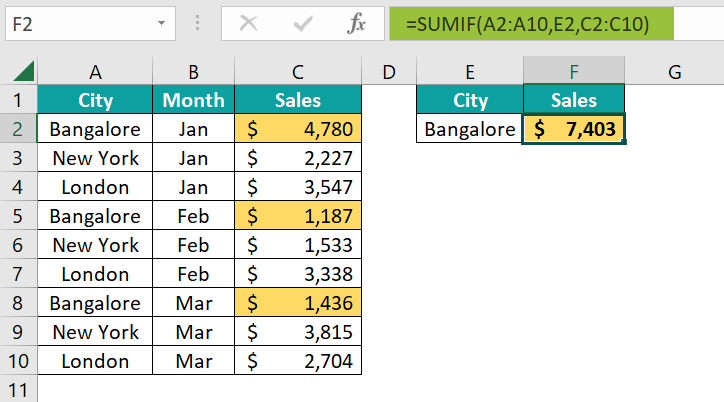
The SUMIF function adds all the colored cells and returns the result as $7,403.

#8 – CONCATENATE Formula in Excel

CONCATENATE function in Excel is used to combine two or more cell values into one cell value.

The syntax of the CONCATENATE function is,

The arguments of the CONCATENATE function are,

• text 1: The first text value that we need to combine. It is a mandatory argument.
• [text 2]: The second text value that we need to combine with text 1. It is an optional argument.

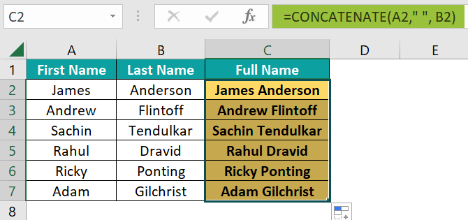
To demonstrate the use of the CONCATENATE function, we have the following data in Excel. We have the first and last names in columns A & B, respectively. In column C, we need to combine both first and last names using the CONCATENATE function.

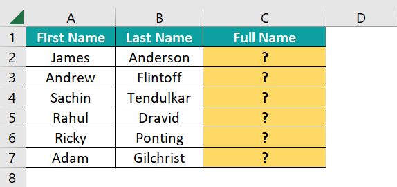
• Step 1: Enter the CONCATENATE function in cell C2, =CONCATENATE(

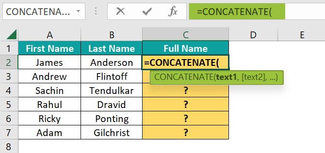
• Step 2:Choose the first text as cell A2.

• Step 3: Choose the second text as cell B2.

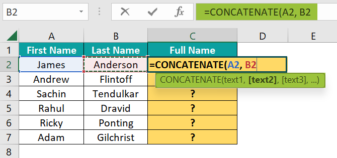
• Step 4: Close the bracket and press “Enter”.

The result we are getting is two names together. However, we need to concatenate space characters that can separate the first and last names.

Before we select the second text as cell B2, enter space in double quotes, and then 3^rd text will be cell B2. The complete formula is =CONCATENATE(A2,” “,B2). Now, drag the formula for the rest of the cells using the excel fill handle.

#9 – LEFT, MID, RIGHT Formula in Excel

Text functions are so useful in Excel, and the important text functions are:

LEFT: It will fetch the required number of characters from the left side of the given text.

MID: It will fetch the required number of characters from the middle of the given text by using the starting position and length.

RIGHT: It will fetch the required number of characters from the right side of the given text.

For instance, we have the following name in Excel.

We will extract the first name, middle name, and last name.

• To extract the first name “Mahendra”, we need to use the LEFT excel function.

• The text will be cell A2, and the number of characters for the first name is 8.

From the left side of the given text, it has extracted 8 characters.

• Similarly, for the middle name, we will use the MID excel function.

• The text will be cell B2, starting number will be 10, and the number of characters will be 5.

• Next, to extract the last name, we will use the RIGHT excel function.

• From the right side of the text number of characters required is 5.

#10 – OFFSET Formula in Excel

The OFFSET excel function is a lookup and reference function in Excel that returns a reference to a cell or range of cells that are offset from the desired cell by a specified number of rows and columns.

The syntax of the OFFSET function is,

The arguments of the OFFSET function are,

• reference: It is the reference of the cell from where we need to start the offset. It is the starting point of the offset. It is a mandatory argument.
• rows: The number of rows to move up or down from the starting point. If we mention a positive number, it will move down from the starting position, and if we mention a negative number, it will move up from the starting position. It is a mandatory argument.
• cols: The number of columns to move to the right or left from the starting point. If we mention a positive number, it will move to the right from the starting position, and if we mention a negative number, it will move to the left from the starting position. It is a mandatory argument.
• [height]: The number of rows we need to return in the returned reference. It is an optional argument.
• [width]: The number of columns we need to return in the returned reference. It is an optional argument.

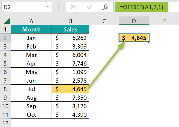
We have the following data in Excel. Assume that we need to fetch the value of the month of Jul starting from cell A1.

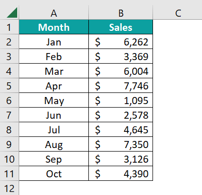
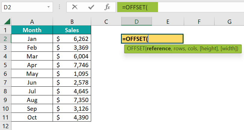
• Enter the OFFSET function in any of the cells.

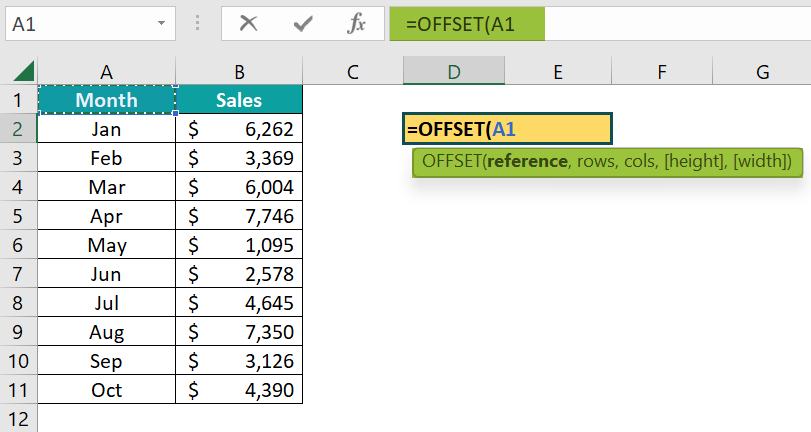
• Reference will be starting position, so enter cell A1 reference.

• We need to fetch the value of the month of Jul, so we need to go down 7 cells. So, enter 7.

• Now the reference will reach cell A8 because we moved down 7 cells. Next, to fetch the sales value, we need to move 1 column to the right, so enter 1 for the cols argument.

• Close the bracket and press “Enter” to get the Jul month sales.

Download Template

This article must help understand the List of Top 10 Advanced Excel Formulas withformulas and examples. You can download the template here to use it instantly.

Recommended Articles

Guide to Advanced Excel Formulas. Here we understand the top 10 advanced excel formulas, step-by-step examples & downloadable excel template. You can learn more from the following articles –

• Basic Excel Formulas
• Excel Formula Not Working
• FORMULATEXT Excel Function