
HLOOKUP Definition
In Excel, HLOOKUP searches for values in the rows of a defined table array and retrieves the value in the cell where we want it. The “H” in HLOOKUP means horizontal movement, and the “LOOKUP” stands for fetching data from a specific source.
While HLOOKUP searches the value horizontally, VLOOKUP explores the value vertically. However, we mostly deal with the table in vertical order in Excel, so the HLOOKUP function is not popularly used.
A fruit merchant, for example, can keep track of the number of oranges. The lookup value, or quantity, is displayed in column B1, the table array is the entire table A1:B3, the row index number is 2, and the range lookup is set to FALSE to retrieve the exact match.
=HLOOKUP(B1,A1:B3,2,FALSE)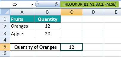
Use this HLOOKUP Template to follow along with the examples in this article.
Download Excel TemplateHLOOKUP() Excel Formula
The syntax of the HLOOKUP formula in Excel is shown in the image below:

Here is an explanation of the arguments accepted by the function:
- lookup_value= It is the value searched in the table’s topmost row.
- table_array= It is the reference or name of the table array from which the data is fetched. The lookup value must be in the topmost row of the table.
- row_index_number= The row no. in the table_array to match and return the value. If row_index_number equals 1, it will return the value from the table_array’s topmost row. Likewise, if row_index_number equals 2, it will return the value from the table_array‘s second row, and so on.
- range__lookup = It is the range that looks up if the value is TRUE or FALSE. TRUE (that is 1) stands for the approximate match. Whereas FALSE (0) stands for the exact match value. If neither happens, the function returns the “#N/A” error.
How To Use HLOOKUP() in Excel?
Let’s look at some HLOOKUP examples to understand better how to use the formula:
Example #1
The image below depicts school data of class 6 students, including students’ names, subjects, and marks. Here, we will attempt to retrieve Tia’s marks in Physics using the HLOOKUP function.
In the table, the data is reflected as below: –
- Column A shows Subjects
- Column B contains marks of John
- Column C contains marks of Tia
- Column D contains marks of Ron
- Column E contains marks of Harry

The steps to retrieve marks of Tia in Physics are as follows:
Step 1: First, we will choose the cell where we want the result to show up. Cell D9 would be the cell in this case.
Step 2: Next, start by entering the lookup value (Tia) that needs to be searched from the topmost row. Since Tia is present in cell C1, enter C1 as the lookup value.

Step 3: Select the table array which ranges from the starting cell address to the end cell address of the whole table, i.e., A1:E7.

Step 4: Add the row index number from which the value needs to be fetched. Since Physics is present in row no. 5, we will enter the row index number as 5.

Step 5: Set the range lookup value as FALSE, which will give an exact match. The complete formula is:
=HLOOKUP(C1,A1:E7,5,FALSE)

Step 6: After entering each value in the preceding step, press the “Enter” key. The results are shown in cell D9 of the image below. Here, the HLOOKUP function retrieved the exact match of Tia’s Physics marks, i.e., 45, from the given table array.

Example #2
The image below depicts the boxes kept in the warehouse and the number of bottles in each box. We will attempt to retrieve the table showing the number of bottles in a particular box using the HLOOKUP function.
In the table, the data is reflected as below:
- Column A contains Boxes
- Column B contains the number of Bottles

The steps to retrieve the number of bottles in a particular box are as follows:
Step 1: To retrieve the desired results, enter the following formula in cell B9.
=HLOOKUP(B1,A1:B5,2,0)
Therefore, start by entering the lookup value that needs to be searched from the topmost row. For example, since we are fetching the number of bottles in cell B1, enter B1 as the lookup value.

Step 2: Select the table array which ranges from the starting cell address to the end cell address of the whole table, i.e., A1:B5.

Step 3: Add the row index number from which the value needs to be fetched. Since the bottles count is present from row no. 2, we will enter the row index number as 2.

Step 4: Set the range lookup value as FALSE or 0, giving an exact match. The complete formula is:
=HLOOKUP(B1,A1:B5,2,0)

Step 5: After entering each value in the preceding step, press the “Enter” key. The results are shown in cell B9 of the image below. You can see that the HLOOKUP function retrieved the exact match of the number of Box1, i.e., 3, from the given table array.

Step 6: Press the “Enter” key. Then, drag the formula downwards till cell B10.

Example #3
Stella selling different fruits can use the HLOOKUP function with the MATCH excel function to track their quantity and price. Then, she can enter the stock details in an Excel sheet and proceed further.
In the table, the data is reflected as below:
- Row 1 contains Fruits
- Row 2 contains the number of fruits
- Row 3 contains the price of fruits

The steps to retrieve the price of the fruits are as follows:
Step 1: To retrieve the desired results, enter the following formula in cell B6.
=HLOOKUP(B5,B1:E3,MATCH(A6,A1:A3,0),FALSE)
Therefore, start by entering the lookup value that needs to be searched from the topmost row. For example, since we are fetching the price of the fruits in cell B5, enter B5 as the lookup value.

Step 2: Select the table array which ranges from the starting cell address to the end cell address of the whole table, i.e., the cell references, B1:E3.

Step 3: Since we have combined the MATCH function with the HLOOKUP function, the match lookup value we will enter is A6.

Step 4: Select the table array which ranges from the starting cell address to the end cell address of the matched data, i.e., A1:A3 of the MATCH function.

Step 5: Set the match type value as 0, which will give an exact match of the MATCH function.

Step 6: Set the range lookup value as FALSE or 0, which will give an exact match of the HLOOKUP function. The complete formula is:
=HLOOKUP(B5,B1:E3,MATCH(A6,A1:A3,0),FALSE)

Step 7: After entering each value in the preceding step, press the “Enter” key. The results are shown in cell B6 of the image below. You can see that the HLOOKUP function retrieved the exact match of Apple’s price, i.e., 300, from the given table array.

Step 8: Press the “Enter” key. Then, drag the formula towards the right till cell E6.

Example #4
The following image shows the data of a hotel and the various services that it offers. Using the HLOOKUP function, we will find the level of their services.
- Column A contains the Category of the hotel departments
- Column B contains the Rating of the departments
- Column C contains the Level value
The HLOOKUP function fetches the value of the level according to the rating done. It brings the value from other rows. Here, we can check multiple lookup values. All the rating values from the B3 to B7 cells are looked up in the given table array A9:F10, which has rating and level values in the row index number is 2. The range lookup value is set as FALSE to fetch the exact match.
=HLOOKUP(B$3:B$7,A$9:F$10,2,FALSE)

The “$” sign is used when the row address of each cell is to be kept locked. Then, when the formula is dragged down, it gives the correct output.

When To Use?
- The HLOOKUP function is used in educational institutions to fetch marks, merits, etc., of students.
- Companies also use it to fetch employees’ performance and salary status.
- Furthermore, it is used in businesses to track different commodities or stocks, performance, etc.
- HLOOKUP function lets you look up the value in horizontal order across the table array with all the data to find the exact or approximate match.
Important Things To Note about HLOOKUP In Excel
- HLOOKUP in Excel finds the value from the table’s topmost row.
- The lookup_value used in the HLOOKUP function must be the exact value in the table_array.
- Also, the lookup_value must be in the first row.
- Note that the whole table_array must be selected from where the value is fetched.
- The row_index_number should always be at the topmost row of the table_array.
- The range_lookup argument is optional, but it should be specified for the output needed – exact match (FALSE) or approximate match (TRUE).
- In the case of any error in the formula or result, it will generate a “#N/A” error.
- Ensure that the reference cell given in the function is correct.
- Do not forget that the HLOOKUP function can only fetch data from top to bottom, not from bottom to top.
- The data structure in the data table should always be horizontal to apply the function.
Frequently Asked Questions (FAQs)
The HLOOKUP in Excel is used to fetch the value from any table. It looks up for the value in the horizontal direction from the table in the same or a different spreadsheet. The function works by using a predefined formula in Excel.
The HLOOKUP formula in Excel to fetch a value from the table is:
=HLOOKUP(lookup_value,[table_array],[row_index_number],[range_lookup])
For example, a fruit vendor can track the quantity of oranges from the given table.
The lookup value, i.e., quantity, is shown in column B1, the table array is the whole table A1:B3, the row index number is 2, and the range lookup is set as FALSE to fetch the exact match.
=HLOOKUP(B1,A1:B3,2,FALSE)
– HLOOKUP in Excel is used to fetch the value from the topmost row of the table and wherever needed.
– It looks up the value horizontally from the same or another spreadsheet of the same workbook or different.
– It reduces the time of searching the value if the table is of n number of rows and columns.
– This function of Excel is very efficient and accurate.
Use this HLOOKUP Template to follow along with the examples in this article.
Download Excel Template
Comments are closed.