
What Is LEFT Function In Excel?
The LEFT Function in Excel is a text function that returns the number of characters from the beginning of the string, i.e., from the left. The LEFT function is an inbuilt function in Excel. It is part of the Excel Text Functions in the Formulas tab.
For example, consider cell A1 with the text string, Peter. Now, let us understand how LEFT Function in Excel works with the following steps.

- The steps required to use LEFT function in Excel are as follows:
- First, select the cell where we want to display the result. In this case, select cell B1.
- Next, type the LEFT Function in cell B1. The formula is =LEFT(A1). Then, press Enter key.
We can see that the function has returned the output as ‘P,’ which is the first character of the entered string while taken from the left.

Use this LEFT Function in Excel Template to follow along with the examples in this article.
Download Excel TemplateKey Takeaways
- LEFT Function in Excel is a function that fetches a substring from a string, starting from the left side.
- The formula of LEFT function in excel is =LEFT(text,[num_char) where,
- text is a mandatory argument that denotes the text string from which we fetch the characters.
- num_chars is an optional argument that indicates the number of characters.
- The #VALUE! error occurs if the given value to the num_chars argument is not 1 or less than 0.
- If there are any extra spaces in the formula, the obtained value might have an error or the result might be incorrect.
LEFT( ) Excel Formula
The syntax of the LEFT Function in Excel, along with the arguments, are as follows:

where,
- text: It is a mandatory argument and denotes the text string from which we fetch the characters.
- num_chars: It is an optional argument indicating the number of characters we want to fetch.
How To Use LEFT( ) In Excel?
Let us understand the two ways to use LEFT function in Excel.
1. Access Left Function from the Excel ribbon
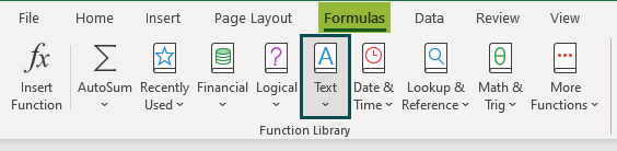
- Go to the Formulas
- Click on the Text option from the Function Library group

- Choose the LEFT function from the drop-down list.

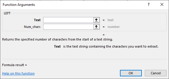
- A window called Function Arguments pops up.
- Enter the arguments in the Text & Num_chars boxes.

- Click OK.
2. Enter the worksheet manually
- Select an empty cell for the output.
- Type =LEFT( in the selected cell.
Alternatively, type =L and double-click the LEFT Function from the list of suggestions shown by Excel.

- Enter the arguments as cell references or direct values.
- Close the parenthesis and press the Enter key.
For example, the below image shows text string values in cell A2. We need to use the following steps to understand LEFT Function in Excel.

The steps used to find values using LEFT Function in excel are as follows:
Step 1: To begin with, select an empty cell for the output. We have selected cell B2 in this case.

Step 2: Next, start by entering the formula in cell B2.
Step 3: Then, we should select the cell having the text. So, in this example, the selected cell is A2.
The complete formula is =LEFT(A2).

Step 4: Press Enter key.
We can see that the function has returned the value ‘A’ in cell B2, which is the first character from the left side of the string.

Thus, the LEFT function returns the values in excel.
Examples
Example #1 – Extracting A Substring Before A Certain Character
The below table shows the first names of people in column A. Now, we need to use the following steps to learn how to use Left function in Excel with the SEARCH function to fetch a substring before space between the two strings.

The steps to demonstrate the LEFT Function are as follows:
Step 1: First, select an empty cell for the output. We have selected cell B2 in this case.
Step 2: Next, start by entering the formula in cell B2.
Step 3: Select the cell reference with the cell having the text string.
So, in this example, select cell range A2:A3.

Step 4: Enter the SEARCH formula with a blank space.

So, the complete formula is =LEFT(A2:A3,SEARCH(“ ”,A2:A3)).

Step 5: Press Enter key.

We can see that the first name, ‘John’ is displayed in cell B2, i.e., the first name from the left side of the string before the space is fetched as output.
Step 6: Simply drag the arrow key to cell A3 to display the result in B3.

Likewise, we can use LEFT function to obtain output in Excel.
Example #2 – Removing the last N characters from a String
The below table shows the text string in cell A2. We need to use the below steps to learn how to use Left function in Excel with the LEN function to remove the last specified number of characters from the string.

The steps to use the LEFT Function are as follows:
Step 1: To begin with, we should select an empty cell to display the output.
In our example, let us select cell B2.

Step 2: Next, enter the formula in cell B2.

Step 3: Now, select the cell having the text string. In this example, the selected cell is A2.

Step 4: Enter the LEN formula and the cell reference whose length is checked. Again, in this example, the selected cell is A2.

Step 5: Now, we need to enter the number of characters we want to eliminate from the string. Here, ‘9’ will be the num_char value.
So, the complete formula is =LEFT(A2,LEN(A2)-9).

Step 6: Press Enter key.
We will be able to see the text string, ‘Time and Tide wait’ in cell B2. Here, the last nine characters from the right side of the string are eliminated.

Similarly, we can use the LEFT function to display our desired output.
Example #3 – Force the Excel LEFT Function to return a Number
The following table shows the text string in cell A2. We need to use the below steps to obtain the values using LEFT Function in Excel with the VALUE function to fetch only numbers.

The steps to use the LEFT Function are as follows:
Step 1: We should select an empty cell for the output. We have selected cell B2 in this case.
Step 2: Next, start by entering the formula in cell B2.
Step 3: Enter the VALUE formula along with the LEFT formula.
Step 4: Select the cell having the text. In this example, the selected cell is A2.

Step 5: Enter the number of digits we want to fetch as a number. In this case, the num_char value will be 3.
The complete formula is =VALUE(LEFT(A2,3)).

Step 6: Press Enter key.

We can see that the function has returned the output (111) in cell B2.
Remember, the VALUE function will only fetch the numeric value in the string according to the number of digits entered in the formula.
LEFT( ) Excel Not Working
The LEFT Function in Excel may not work for the following reasons.
- The num_chars argument is less than zero: The num_char value should not be less than 0; if so, the LEFT Function will return #VALUE!
- Also, the error occurs when the num_char argument is replaced by any other function.
For example, consider the table with the text ‘Papaya’ in cell A1.
Here, assume that we want to display the result in cell B1. So, insert the LEFT Function in cell B1 with the num_char value less than ‘1’.
The complete formula is =LEFT(A1,-1).

Press Enter key.

Clearly, we can see that the output returned by the function has #VALUE! error.
- Leading spaces in the original text: When the data is copied from other sources, sometimes the leading spaces may be left, which returns the wrong output or errors. For instance, assume that if we copy the text in cell A1 by mistake, some leading spaces are also copied. Then, when we apply the LEFT Function, the function will either return an error or displays incorrect output.
- Excel LEFT Function does not work with Dates-: The LEFT Function reads the individual part of a date, such as a day, month, or year. It will retrieve the first few digits of the number that represents that date. For example, we enter the date in cell A1 and then apply the LEFT Function. The dates in excel have numeric values, so the function will not work on the dates. The function will return an error or show an incorrect output.
Important Things To Note
- The LEFT Function in Excel formula returns a value that can be a string or text.
- The LEFT Function in Excel is used for extracting characters starting from the left side of the text.
- The num_of_chars argument (one of the two arguments) value is optional, and the default value is set to 1.
- The function returns #VALUE! Error if the default value is altered.
- The LEFT Function in Excel extracts digits from numbers as well.
Frequently Asked Questions (FAQs)
The LEFT Function in Excel extracts the character from the left side of the string based on the argument.
The formula of the LEFT Function is =LEFT(text,[num_char)
For example, consider cell A1 with the text string ‘Calendar’. Let us understand how LEFT Function in Excel works with the following steps.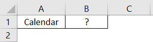
The steps required to use LEFT function in excel are as follows:
Step 1: Select the cell where we want to display the result. In this case, select cell B1.
Step 2: Type the LEFT Function in cell B1.
The formula is =LEFT(A1).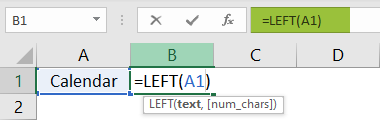
Step 3: Press Enter key.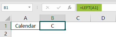
We can see that the function has returned the output as ‘C,’ which is the first character of the entered string while taken from the left.
Thus, we can easily use the LEFT function in excel to find values.
The LEFT Function in Excel is used when we want to fetch the specific characters from the left side of the text string.
We can manually type the LEFT Function in Excel function in the desired cell or use the following steps:
1. Select the cell which has the number.
2. Select the Formulas tab.
3. Click on the Text option.
4. Select the LEFT option from the drop-down list.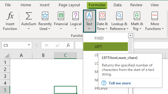
5. The Function Arguments window pops up.
6. Enter the value in the Text and num_chars arguments.
7. Click OK.
Use this LEFT Function in Excel Template to follow along with the examples in this article.
Download Excel Template