
What Is ROUND Function In Excel?
In Excel, the ROUND Function rounds up a given number to the specified number of digits. It is one of the inbuilt Math and Trigonometry functions. There are two functions available in the ROUND function group; they are ROUNDUP and ROUNDDOWN functions. Unlike the other two functions, the ROUND function rounds up a number both up and down.
For example, consider the below table with the value 220.666 in cell A1. Now, let us learn how to use Round Excel function to round up a number.

The steps used to obtain a rounded value in Excel are as follows:
Step 1: First, we must select an empty cell to display the result. So, let us select cell B1.
Step 2: Next, enter the formula =ROUND(A1,0) in cell B1.
Step 3: Then, press Enter key.
Clearly, the value 220.666 is rounded as 221.

- Therefore, we can use Round Excel function to get rounded values.
Use this ROUND Excel Function Template to follow along with the examples in this article.
Download Excel TemplateKey Takeaways
- The ROUND function in Excel rounds a number according to the number of digits allotted in the argument.
- The ROUND function group has two more functions (ROUNDUP and ROUNDDOWN functions).
- The ROUND function always returns numeric values.
- The formula of the ROUND function is =ROUND(number,num_digits) where –
- Positive digits (1, 2, and 3) rounds the decimals in that location.
- Negative digits (like -1,-2, and -3) round the decimals according to the multiples of 10, 100, and 1000.
- ‘0’ rounds the number based on the nearest number.
ROUND( ) Excel Formula
The syntax of the ROUND Excel Function is:

Both the arguments in the ROUND function are mandatory.
- number: It denotes the numerical value which we want to round up or down.
- num_digits: It mentions the location at which the number is rounded.
Meanwhile, the following table shows the digits and the reference with which the values are rounded.
| Digits | Result |
|---|---|
| 0 | Round to the nearest number |
| 1 | Round the 1st decimal number to the right |
| 2 | Round 2 decimal numbers to the right |
| 3 | Round 3 decimal numbers to the right |
| -1 | Round to the nearest 10 |
| -2 | Round to the nearest 100 |
| -3 | Round to the nearest 1000 |
How To Use ROUND Function?
Let us learn how ROUND function works in Excel using the following example.
The below table shows the input values in column A. Now, we need to find the round values using the ROUND Excel Function.

The steps used to round the values are as follows:
Step 1: First, we should choose a blank cell to display the result. In our example, let us select Column B.
Step 2: Next, enter the formula, =ROUND( in cell B2.
Now, we should select the cell that contains the number. So, let us select cell A2.
Step 3: Then, we need to specify the digit to round the values.
In our example, let us round to the nearest number. So, type ‘0’ in the second argument.
Thus, the complete formula is =ROUND(A2,0).

Step 4: Press Enter key.
Clearly, we can see that the function has returned the value 325 in cell B2.

Step 5: Similarly, we can use the ROUND function formula in cells, B3 and B4, or we can use the Autofill option.
Let us use the AutoFill option. Drag the cursor down to cell B4.
Automatically, Excel returns the values in cells B3 and B4, as shown in the image below:

- Therefore, we can use Round Excel function to get rounded values.
Examples
Example 1: Using Num_Digit (1)
The below table shows the input values in column A. Now, we need to find the rounded values of the numbers. Let us see how Round function works in Excel.

The steps used to find the rounded values are as follows:
Step 1: To begin with, we should choose a blank cell to display the result. In our example, let us select column B.
Step 2: Next, enter the formula =ROUND( in cell B2.
For the first argument, we should select the cell that contains the number. So, let us select cell A2.

Step 3: Then, we need to specify the digit to round the values.
In our example, let us round the first decimal number. So, type ‘1’ in the second argument.
Thus, the complete formula is =ROUND(A2,1).

Step 4: Next, press Enter key.
The function has returned the value 125.0 in cell B2.
It is because the ROUND function formula has rounded the first decimal value. So, instead of 124.9, the result is obtained as 125.0.

Step 5: Similarly, we can use the ROUND function formula in cells B3 and B4. Alternatively, we can also use the autofill option.
For our example, let us use the AutoFill option. Drag the cursor down to cell B4.
Excel automatically returns the values in cells B3 and B4, as shown in the image below:

- Therefore, we can use Round Excel function to get rounded values.
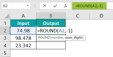
Example 2: Using Num_Digit (-1)
The table below shows the input values in column A. Let us learn how to use Round function in Excel to round up the number using -1.

The steps used to find the rounded values are as follows:
Step 1: First, we should choose a blank cell to display the result. In our example, let us select column B.
Step 2: Then, enter the formula =ROUND( in cell B2.
For the first argument, we should select the cell that contains the number. So, let us select cell A2.

Step 3: Next, we need to specify the digit to round the values.
In our example, let us round the first decimal number. So, type ‘-1’ in the second argument.
So, the complete formula is =ROUND(A2,-1).
Step 4: Then, press Enter key.
Clearly, we can see that the function has returned the value 70 in cell B2. It is because -1 in the ROUND function rounds the value based on the nearest multiple of 10.

Step 5: Similarly, we can use the ROUND function formula in cells B3 and B4 or we can use the autofill option.
In this example, let us use the AutoFill option. Drag the cursor down to cell B4.
Excel automatically returns the values in cells B3 and B4, as shown in the image below:

- Therefore, we can use Round Excel function to get rounded values.
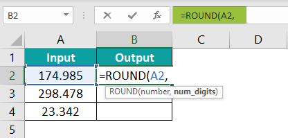
Example 3: Using Num_Digit (2)
The table below shows the input values in column A. Now, we need to find the rounded values of the numbers. Let us see how Round function works in Excel.

The steps used to find the rounded values are as follows:
Step 1: To begin with, we should choose a blank cell to display the result. In our example, let us select column B.
Step 2: Next, enter the formula =ROUND( in cell B2.
For the first argument, we should select the cell that contains the number. So, let us select cell A2.
Step 3: Also, we need to specify the digit to round the values.
In our example, let us round the first decimal number. So, type ‘2’ in the second argument.
So, the complete formula is =ROUND(A2,2).

Step 4: Then, press Enter key. The function has returned the value 175.0 in cell B2.
Clearly, the ROUND function formula has rounded the values to the right. So, instead of 174.985, the result is obtained as 175.0

Step 5: Similarly, we can use the ROUND function formula in cells B3 and B4, or we can use the autofill option.
Let us use the AutoFill option. So, drag the cursor down to cell B4.
Automatically, excel returns the values in cells B3 and B4, as shown in the image below:

- Therefore, we can use Round Excel function to get rounded values.
Example 4: Using Num_Digit (-2)
The table below shows the input values in column A. Now, let us learn how to use Round function in Excel to round up the number using -2.

The steps used to find the rounded values are as follows:
Step 1: First, we should choose a blank cell to display the result. In our example, let us select column B.
Step 2: Next, enter the formula =ROUND( in cell B2.
For the first argument, we should select the cell that contains the number. So, let us select cell A2.

Step 3: Then, we need to specify the digit to round the values.
In our example, let us round the first decimal number. So, type ‘-2’ in the second argument.
So, the complete formula is =ROUND(A2,-2).

Step 4: Finally, press Enter key.
Clearly, we can see that the function has returned the value 100 in cell B2. It is because -2 in the ROUND function rounds the value based on the nearest multiple of 100.

Step 5: Similarly, we can use the ROUND function formula in cells B3 and B4, or we can use the autofill option.
Let us use the AutoFill option. So, drag the cursor down to cell B4.
Excel automatically returns the values in cells B3 and B4, as shown in the image below:

- Therefore, we can use the Round Excel function to get rounded values of the supplied numbers.
Important Things To Note
- The ROUND function rounds the values both up and down. Other ROUND functions include they are ROUNDUP and ROUNDDOWN.
- Also, the ROUND function works by rounding the numbers to the specified digit.
- If the number of digits mentioned in the second argument is –
- Higher than ‘0’, the function rounds the values to the right.
- Equal to ‘0’, it rounds to the nearest number.
- Lesser than ‘0’, the function rounds the values to the left. -1, -2 and -3 rounds the number based on the multiples of 10, 100, and 1000 respectively.
Frequently Asked Questions (FAQs)
Typically, the ROUND function is used in Excel to round up the numerical data according to the number of digits assigned to round the values.
The ROUND function formula is =ROUND(number, num_digits)
The steps used to find the rounded values in Excel are:
● Select an empty cell to display the result.
● Type the formula =ROUND(….
● Select the cell with the value along with the number of digits.
● Press ENTER.
For example, consider the below table with the value 789.0912 in cell A1. Now, let us learn how to use round function in excel to round up the number. 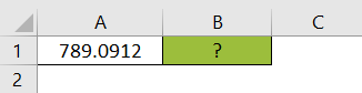
The steps used to obtain a rounded value in Excel are as follows:
Step 1: First, we must select an empty cell to display the result. So, let us select cell B1.
Step 2: Next, enter the formula =ROUND( in cell B1.
For the first argument, we should select the cell that contains the number. So, let us select cell A1.
Step 3: Then, we need to specify the digit to round the values.
In our example, let us round the first decimal number. So, type ‘3’ in the second argument.
So, the complete formula is =ROUND(A2,3).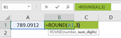
Step 4: Now, press Enter.
In just a few steps, we can see that the value 789.0912 is rounded as 789.091.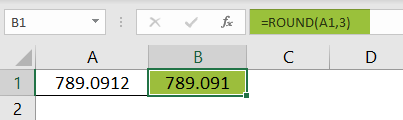
❖ Therefore, we can use Round Excel function to get rounded values.
We can manually write the formula or use the following steps to use ROUND Excel Function;
1. To begin with, select the cell which has the number.
2. Then, choose the Formulas tab.
3. Next, click on the Math & Trig option from the Function Library group.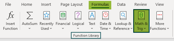
4. And, select the ROUND option.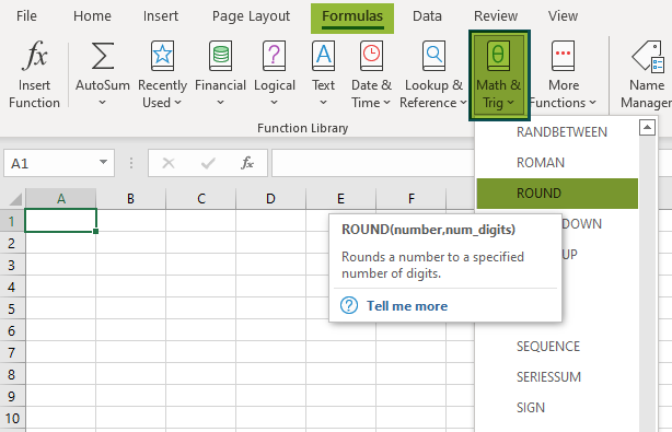
5. In some time, the Function Arguments window pops up.
6. Here, enter the value in the Number and Num_digits as the number of arguments.
7. Finally, click OK.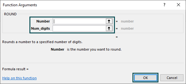
Use this ROUND Excel Function Template to follow along with the examples in this article.
Download Excel Template