SEARCH Function in Excel

What Is SEARCH Function In Excel?

The SEARCH Function in Excel is one of the important in-built functions of MS Excel. The function is available in the Text group under the Function Library. The SEARCH Function is used to locate or find one string in the second string; Similarly, the function will locate a search text in the string. The Search function allows special characters (like:? *, ~), and the function is not case-sensitive.

For example, consider the below table with the text string in cell A1. Now, we need to use the below steps to obtain the result using SEARCH function.

The steps used to find the output using SEARCH function are as follows. First, select the cell to display the result. In this example, we have selected cell C2. Next, enter the SEARCH function in excel formula in cell C2. The complete formula is =SEARCH(B2,A2,1). Then, press Enter key.

We can clearly see that the function has returned the value as 4 in cell C2. Similarly, with SEARCH function, we can find results in Excel.

What is the SEARCH Function in Excel?

The SEARCH Excel Function formula is =SEARCH(find_text,within_text,[start_num]), where
- find_text and within_text are mandatory arguments and denotes the character or sub-string we wish to search for and the text string that we need to search.
- start_num is the only optional argument that shows the position of the ‘within_text’ string.

Remember, the #VALUE! error occurs if no matching string is found in the “within_text” argument.
The SEARCH Function in excel also uses special characters, i.e., “?”, “*,” and “~” tilde.

SEARCH() Excel Formula

The syntax of the SEARCH Excel Function is

find_text: It is a mandatory argument and denotes the character that is being searched.
within_text: It is also a mandatory argument. It is the text string that we have to search.
start_num: It is the optional argument showing the position of the ‘within_text’ string. It shows the position from which the function begins the search. Since it is an optional argument, if the users ignore this argument, the function automatically takes the default value of 1.

Excel VBA – All in One Courses Bundle (35+ Hours of Video Tutorials)

If you want to learn Excel and VBA professionally, then Excel VBA All in One Courses Bundle (35+ hours) is the perfect solution. Whether you’re a beginner or an experienced user, this bundle covers it all – from Basic Excel to Advanced Excel, Macros, Power Query, and VBA.

Start Learning Now

How To Use SEARCH Excel Function?

We can insert SEARCH Function with the below two methods.

#1 – Access From The Excel Ribbon

Choose the empty cell which will contain the result.
Go to the Formulas tab and click it.
Select the Text option from the drop-down menu.
Select SEARCH from the menu.
A window called Function Arguments appears.
Based on the number of arguments, enter the value in the find_text, within_text, & start_num.
Select OK.

#2 – Enter The Worksheet Manually

Select an empty cell for the output.
Type =SEARCH( in the selected cell. Alternatively, type =S and double-click the SEARCH function from the list of suggestions shown by Excel.
Press the Enter key.

The succeeding example depicts the strings, and we will calculate the output using the SEARCH function.

The below table shows text strings and searches text values in columns A and B. We need to use the below steps to calculate the output using SEARCH function in Excel.

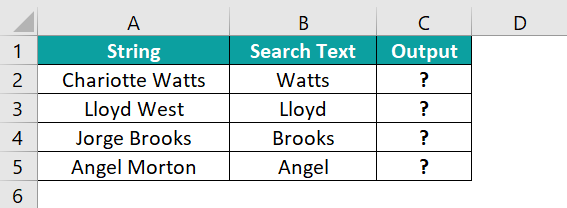
How to use SEARCH Excel Function - Basic Example

The steps to find the values using SEARCH Function in Excel are as follows:

To begin with, select the cell where we will enter the formula and calculate the result. The selected cell, in this case, is cell C2.
Next, we will enter the SEARCH formula in cell C2
Enter the value of ‘find_text’ as B2, i.e., the text value we need to find.
Enter the value of ‘within_text’ as A2, i.e., the string in which the text value is searched.
Enter the value of ‘start_num’ as 1, i.e., the starting position in the string.
The complete formula is =SEARCH(B2,A2,1) in cell C2.
Press Enter key.

We can see that the function has returned the results as 11, as shown in the image below.
Press enter and drag the cursor to cell C5, as shown in the following image.

Similarly, with SEARCH function in Excel, we can fetch the output.

Examples

Example #1

The following table shows ID and search text in columns A and B. We need to use the below steps to obtain the result using SEARCH function in excel.

The steps to evaluate the values with SEARCH Function are as follows:

Step 1: Select the cell where we will enter the formula and calculate the result. The selected cell, in this case, is cell C2.

Step 2: Next, we will enter the SEARCH formula in cell C2.

Step 3: Enter the value of ‘find_text’ as B2, i.e., the text value we need to find.

Step 4: Enter the value of ‘within_text’ as A2, i.e., the string in which the text value is searched.

Step 5: Enter the value of ‘start_num’ as 1, i.e., the starting position in the string.

Step 6: The complete formula is =SEARCH(B2,A2,1)in cell C2.

Step 7: Press Enter key.

We can see that the function has returned the results in cell C2 as 11, as shown in the image below.

Step 8: Press enter and drag the cursor to cell C5.

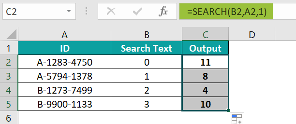
Likewise, we can obtain results with SEARCH function in Excel.

Example #2

The following table shows data and search text in columns A and B. We need to use the below steps to obtain the result using SEARCH function.

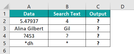
The steps to evaluate the values by the SEARCH Function in Excel are as follows:

Step 1: Select the cell where we will enter the formula and calculate the result. The selected cell, in this case, is cell C2.

Step 2: Next, we will enter the SEARCH formula in cell C2.

Step 3: Enter the value of ‘find_text’ as B2, i.e., the text value we need to find.

Step 4: Enter the value of ‘within_text’ as A2, i.e., the string in which the text value is searched.

Step 5: Enter the value of ‘start_num’ as 1, i.e., the starting position in the string.

Step 6: The complete formula is =SEARCH(B2,A2,1)in cell C2.

Step 7: Press Enter key.

The function returns the result in cell C2 as 3 as shown in the image below.

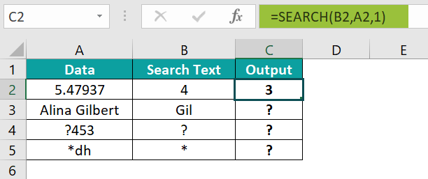
Step 8: Press enter and drag the cursor to cell C5.

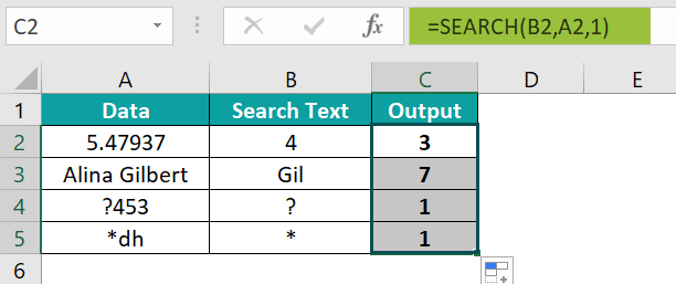
Similarly, we can find results with SEARCH function in excel.

Example #3

The following table shows cities and search text in columns A and B. We need to use the below steps to obtain the result using SEARCH function in excel.

The steps to evaluate the values by the SEARCH Function in Excel are as follows:

Step 1: Select the cell where we will enter the formula and calculate the result. The selected cell, in this case, is cell C2.

Step 2: Next, we will enter the SEARCH formula in cell C2.

Step 3: Enter the value of ‘find_text’ as B2, i.e., the text value we need to find.

Step 4: Enter the value of ‘within_text’ as A2, i.e., the string in which the text value is searched.

Step 5: Enter the value of ‘start_num’ as 1, i.e., the starting position in the string.

Step 6: The complete formula is =SEARCH(B2,A2,1)in cell C2.

Step 7: Press Enter key.

We can see that the function has returned the result in cell C2 as 2.

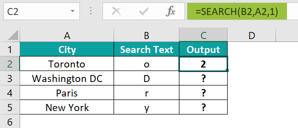
Step 8: Press enter and drag the cursor to cell C5, as shown in the following image.

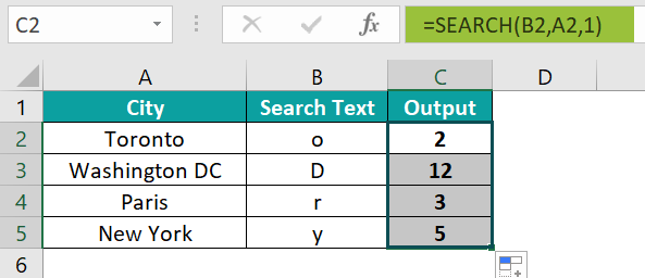
Likewise, using SEARCH function in Excel, we can obtain results.

Important Things To Note

The SEARCH function in Excel is not case-sensitive.
The function always returns an integer value.
It can be used with other formulas and functions.
The FIND function in excel doesn’t support case sensitivity or the use of special characters, but the SEARCH function searches the given data without case sensitivity and uses special characters.
The #VALUE! error occurs if the “start_num” value is greater than the length of the “within_serach” string or not greater than zero while using this function.

Frequently Asked Questions (FAQs)

1. What does the SEARCH function do in Excel?

The SEARCH function in excel will return the position of a specified character or sub-string within a supplied text string. In addition, the function will return an integer value, which represents the position of the search string in the second string.
The syntax of the SEARCH function is
=SEARCH(find_text,within_text,[start_num])

2. How does the SEARCH function work in Excel?

For example, consider the below table with value and search text in columns A and B. We need to use the below steps to obtain the result using SEARCH function in excel.

The steps used to find the output with SEARCH function are as follows:

• Step 1: Select the cell to display the result. In this example, we have selected cell C2.

• Step 2: Enter the SEARCH function in excel formula in cell C2.
The complete formula is =SEARCH(B2,A2,1).

• Step 3: Press Enter key.
We can clearly see that the function has returned the value as 2 in cell C2.

Similarly, we can use SEARCH function in excel.

3. Where is the SEARCH Function in Excel?

We can insert SEARCH Function in Excel using the following steps:
• Choose the empty cell which will contain the result.
• Go to the Formulas tab and click it.
• Select the Text option from the drop-down menu.
• Select SEARCH from the menu.

• A window called Function Arguments appears.
• As the number of arguments, enter the value in the find_text, within_text, & start_num.
• Select OK.

Download Template

This article must help understand the SEARCH Excel Function’s formula and examples. You can download the template here to use it instantly.

SEARCH Function in Excel Download

SEARCH Function in Excel