FIND Function in Excel

What Is FIND Function In Excel?

The FIND function in Excel is used to find the text string in any cell and returns the position of that cell as output. The Find function only takes text format as searched reference. It is the most underrated function of the “Formula” tab under the “Function Library” group.

Let us learn FIND function in Excel with example. Consider the table with the text string in column A. Now, we need to use the below steps to fetch the letter L’s position from the string ‘Excelmojo’ mentioned in column B using the FIND function.

The steps used to fetch the position of a letter in a text string using FIND function in Excel are as follows:

• To begin with, select the cell to display the result.
• Next, enter the FIND formula in cell C2. So, the complete formula is =FIND(B2,A2)
• Then, press Enter key.

Clearly, we can see that the result is returned as 5. It indicates the letter ‘l’ position in the text string.

Likewise, we can use the FIND function in Excel to fetch the letter’s position in the text.

Find() Excel Formula

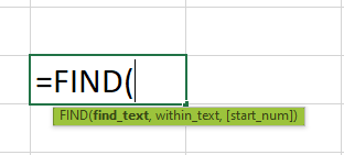
The syntax of the FIND Excel Function is:

where,

• find_text: It is a mandatory argument and denotes the substring or character we are looking to find.
• within_text: It is also a mandatory argument and indicates the string to be searched within.
• start_num: It is an optional argument and shows the position in the within_text string from which the search begins.

How To Use FIND Excel Function?

2. Enter the worksheet manually

• Select an empty cell for the output.
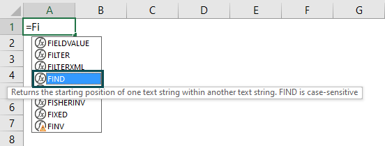
• Type =FIND( in the selected cell.

Alternatively, type =F and double-click the FIND function from the list of suggestions shown by Excel.

• Enter the arguments as cell references in Excel or direct values.
• Close the parenthesis and press Enter

The below table shows the string and search character in columns A and B, respectively. First, we need to find the ‘l’ position using the Find function in Excel.

The steps used to fetch the position of the letter with the FIND function are as follows:

Step 1: To begin with, select an empty cell to display the output. We have selected cell C2 in this case.

Step 2: Next, start by entering the formula in cell C2.

Step 3: Now, enter the find_text value as B2 in cell C2.

Step 4: Then, enter the within_text value as A2 in cell C2.

So, the complete formula is =FIND(B2,A2).

Clearly, the searched character position is shown in C2 as ‘3’.

Likewise, we can use FIND function in excel.

Examples

Example – 1 – Find A Single Character Within A Text String

The following table shows the string and searching character in column A and B. Now, we need to use the below steps to find the position of ‘l’ using Find function in Excel.

The steps used to fetch the position of a letter in the text using FIND function are as follows:

Step 1: First, select an empty cell to display the output. We have selected cell C2 in this case.

Step 2: Next, start by entering the formula in cell C2.

Step 3: Then, enter the find_text value as B2 in cell C2.

Step 4: Now, enter the within_text value as A2 in cell C2.

So, the complete formula is =FIND(B2,A2).

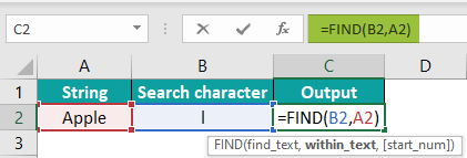
The searched character position is shown in C2 as ‘4’.

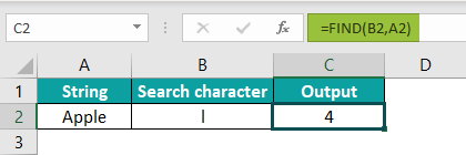
Similarly, we can use the FIND function to fetch the position of a mentioned letter.

Example – 2 – Count The Number Of Times A Single Character Occurs In A Range

Let us learn FIND function in Excel with example.

The below table lists fruits in column A. Next, we need to count the number of times the letter ‘a’ occurs in the range using the FIND function in Excel with SUMPRODUCT and ISNUMBER Excel function.

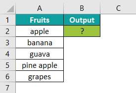
The steps to find the character using FIND function are as follows:

Step 1: First, select an empty cell to display the output. We have selected cell B2 in this case.

Step 2: Next, start by entering the formula in cell B2.

Step 3: Then, enter the Excel SUMPRODUCT formula.

This function will return the unary operator, which becomes an argument of the SUMPRODUCT function.

Remember, the array of numbers is a single array; the SUMPRODUCT will sum it.

Step 4: The unary operator or the double negative symbol (- -) converts every ‘true’ and ‘false’ output of the ISNUMBER function into 1 and 0, respectively. 

Step 5: Then, enter the ISNUMBER formula.

Also, this function will be returned by the FIND function and becomes an argument of the ISNUMBER function.

If the output of the FIND function is numeric, the ISNUMBER returns ‘true,’ and if the production of the FIND function is non-numeric or error, the ISNUMBER returns ‘false.’

Step 6: Next, enter the find_text value as ‘a’ in cell B2.

Step 7: Then, enter the within_text value as A2:A6 in cell B2.

So, the complete formula is =SUMPRODUCT(–(ISNUMBER(FIND(“a”,A2:A6)))).

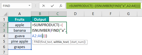
Step 8: Finally, press Enter key.

Clearly, we can see that the function has returned the output as ‘5’. It indicates that the character ‘a’ has appeared in the table range for 5 times.

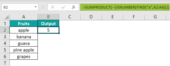
Likewise, we can detect the character’s position using FIND function in excel.

Example – 3 – Count The Text Strings Ending With Certain Characters

The following table shows text strings in column A. Now, we need to find the below steps to count the characters ending with ‘c’ and ‘p’ using the FIND function in Excel with SUMPRODUCT and ISNUMBER functions.

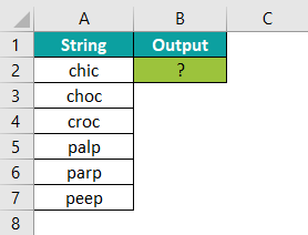
The steps to count the characters using the FIND function in Excel with SUMPRODUCT and ISNUMBER functions are as follows:

Step 1: To begin with, select an empty cell to display the output. We have selected cell B2 in this case.

Step 2: Next, start by entering the formula in cell B2.

Step 3: Then, enter the SUMPRODUCT formula.

This function will return the unary operator, which becomes an argument of the SUMPRODUCT function. The array of numbers is a single array; the SUMPRODUCT will sum it.

Step 4: The unary operator or the double negative symbol (- -) converts every ‘true’ and ‘false’ output of the ISNUMBER function into 1 and 0, respectively. 

Step 5: Next, enter the ISNUMBER formula.

The FIND function will return this function and becomes an argument of the ISNUMBER function. If the output of the FIND function is numeric, the ISNUMBER returns ‘true,’ and if the product of the FIND function is non-numeric or error, the ISNUMBER returns ‘false.’

Step 6: Then, enter the find_text value as ‘c’ and ‘p’ in cell B2.

Step 7: Also, enter the within_text value as A2:A7 in cell B2.

So, the complete formula is =SUMPRODUCT(–((ISNUMBER(FIND(“c”,A2:A7))+ (ISNUMBER(FIND(“p”,A2:A7)))>0)).

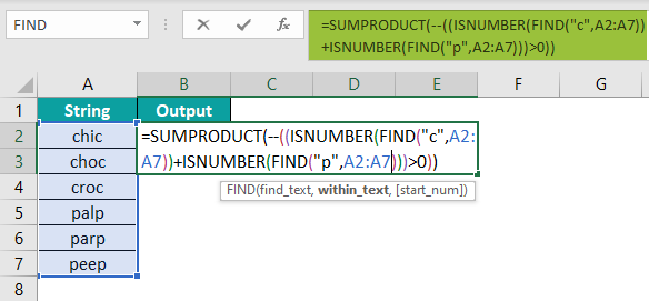
Step 8: Now, press Enter key.

Clearly, the function has returned the number of times the text string ending with ‘c’ and ‘p’ in B2 as ‘6’.

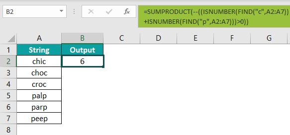
Likewise, we can find the number of times a word has appeared using FIND function in excel.

Example – 4 – Extract Certain Characters From A Cell

The below table shows a text string in cell A2. Now, we will try to extract certain characters from the text string in cell B2.

Since we are looking to extract the characters after the “*” symbol from the middle of the text string present in cell A2, we will be using the FIND function in combination with MID function and LEN Excel function.

The steps to extract certain characters using the FIND function are as follows:

Step 1: Select an empty cell for the output. We have selected cell B2 in this case.

Step 2: Next, enter the above formula in cell B2.

=MID(A2,FIND(“*”,A2),FIND(” “,MID(A2,FIND(“*”,A2),LEN(A2))))

The reasons we use LEN and MID functions here are:

• The MID function checks the string from the middle of the text string.
• The LEN function will count the length of the text string.

Step 3: Enter the find_text value as “*”, as we seek to extract the characters starting with the “*” symbol.

Step 4: Enter the within_text value as A2.

Step 5: Finally, press Enter key.

We can find the result as ‘*someone’ in cell B2.

Explanation:

• The MID function is used to extract certain characters from the middle of the text string present in the cell A2.
• After extracting the certain character from the string, the LEN function will truncate the trailing spaces and strings in the column from the full length.

Likewise, to extract the “*” symbol, the words following it, and the trailing spaces, we can modify the above formula as:

=MID(A2,FIND(“*”,A2),LEN(A2))

Important Things To Note

• The FIND function in Excel helps find the text’s position in a string.
• The function finds if the find_text argument contains two same characters. If so, the function will return the first character’s position.
• The within_text argument of the FIND function in Excel identifies the text within the sample.
• The FIND function in Excel finds if find_text is the empty string, the function gives back the first character in the search string.
• The FIND function returns the #VALUE! Error. It occurs if the find_text value does not exist in within_text, if the start_num contains more characters than within_text, or if the start_num is zero or a negative number.

Frequently Asked Questions

Download Template

This article must help understand the FIND function in Excel with its formula and examples. You can download the template here to use it instantly.

Recommended Articles

This has been a guide to FIND Function in Excel. Here we discuss how to use FIND formula with examples and downloadable excel template. You can learn more from the following articles – 

• Show Formula In Excel
• COUNTIF Excel Function
• DATE Excel Function