COUNTIF Function Definition
The COUNTIF Excel Function counts the cells in a cell range that matches a specific criterion. The function returns the count of the cells with a numerical value, text, dates, etc. The COUNTIF Formula in Excel is an inbuilt function, so we can directly enter the formula in the cell or select it from the “Function Library”.
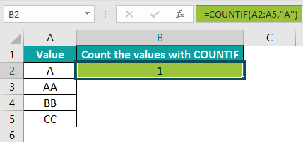
The following image shows the values in Column A. Enter the formula, =COUNTIF(A2:A5,“A”) in cell B2, to count the cells having “A” in the cell range A2:A5. As a result, we will get the following output.
📥Download the ready-to-use Excel template to practice this tutorial yourself.
COUNTIF Excel functionTable of contents
Key Takeaways
- The COUNTIF Excel Function counts the cells with numeric and alphabetic values in a range or array based on the test condition and returns the accurate result.
- When using the function, numerous criteria or test conditions can be specified in a single dataset.
- The “Formulas” > “Function Library” > “More Functions” > “Statistical” menu item provides access to the function.
- One can double-click the COUNTIF function from Excel’s list of suggested functions by typing =C and selecting it from the list, or by typing =COUNTIF( in a cell.
COUNTIF() Excel Formula
The syntax of the COUNTIF formula in Excel is:
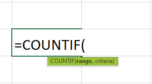
The arguments of the COUNTIF formula in Excel are,
- range – It is a cell range to apply the criteria argument. It is a mandatory argument.
- criteria – It is a condition applied to the cell range with values. It is a mandatory argument.
How To Use The COUNTIF Function In Excel?
We can use the COUNTIF Function in Excel using two methods, namely,
#Method 1 – Access from the Excel Ribbon.
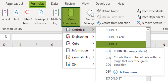
Select the “Formulas” tab > go to the “Function Library” group > select the “More Functions” drop-down > click on the “Statistical” option > select the “COUNTIF” option, as shown below.
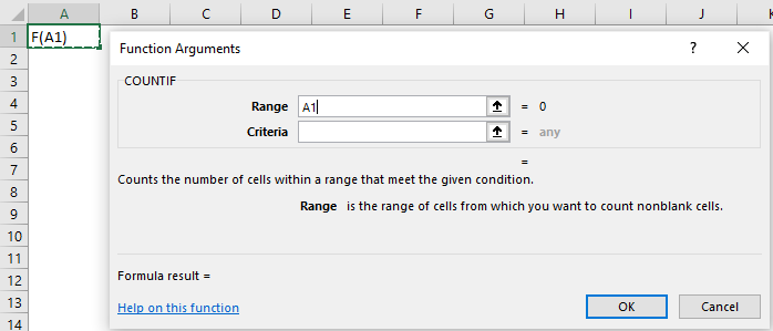
The “Function Arguments” window opens.
Now, enter the values in the “Range” and the “Criteria” fields > click on “OK”.
#Method 2 – Enter the COUNTIF formula in the worksheet manually.
- Select an empty cell for the output.
- Type =COUNTIF( in the selected cell. [Alternatively, type =C and double-click the COUNTIF function from the list of suggestions shown by Excel].
- Enter the arguments as Excel cell references or direct values.
- Close the parenthesis and press the “Enter” key.
Basic Example
We will calculate the types of Pokémon using the COUNTIF Function.
In the table, the data is,
- Column A contains the Name.
- Column B contains the Type.
- Column C contains the Total Status.
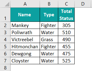
The steps to count the number of cells using the COUNTIF Function in Excel are as follows:
1: First, select Column F for the output.

2: Enter the formula, =COUNTIF(B2:B7,E2) in cell F2.
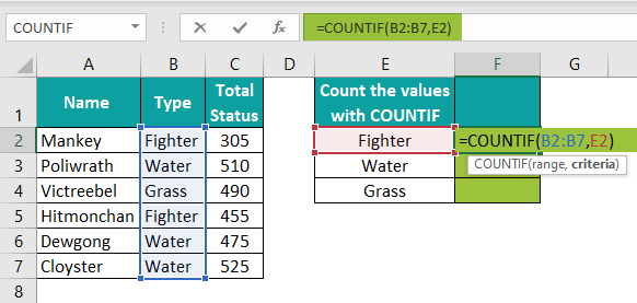
3: Press the “Enter” key. The output is 2 as shown below, i.e., there are 2 Pokémon with the “Fighter” type.

4: Drag the formula from cell F2 to F4 using the fill handle.
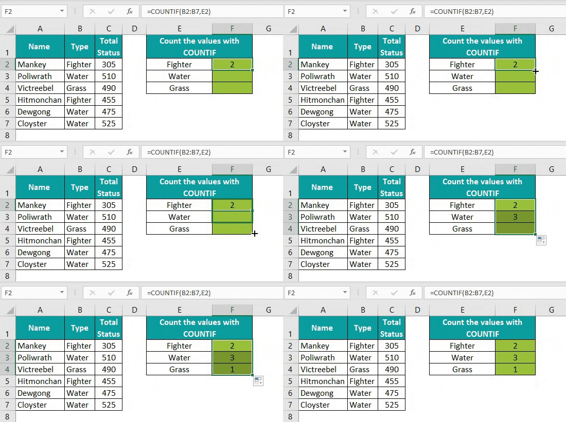
The output is shown above. Therefore, the function counts the Pokémon names in the cell range as per the Pokémon type criteria and returns the count.
Examples
We will understand the COUNTIF Function using advanced scenarios.
Example #1
We will calculate the number of members doing certain tasks using the COUNTIF Function.
In the table, the data is,
- Column A shows the Name.
- Column B contains the Task.

The steps to count the number of cells using the COUNTIF Function in Excel are as follows:
Step 1: First, select Column E for the output.
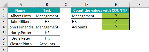
Step 2: Enter the formula, =COUNTIF(B2:B7,D2) in cell E2.
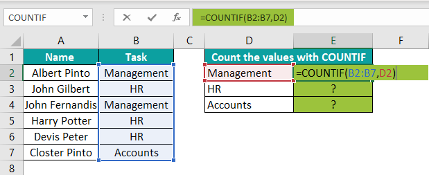
Step 3: Press the “Enter” key. The output is 2 as shown below, i.e., there are 2 members with the “Management” task.

Step 4: Drag the formula from cells E2 to E4 using the fill handle.
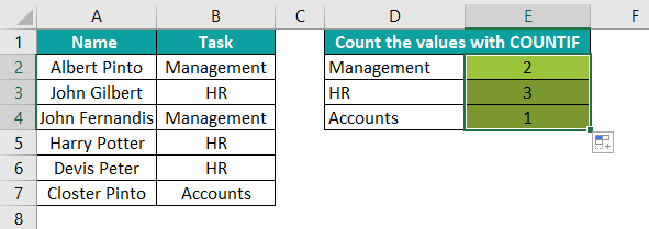
The output is shown above. Therefore, the function counts the Member names as per their Tasks criteria and returns the count.
Example #2
We will calculate the fruits by their names using the COUNTIF Excel Function.
In the table, the data is,
- Column A shows the Fruits.
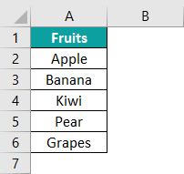
The steps to count the number of cells using the COUNTIF Function in Excel are as follows:
Step 1: First, select Column C for the output.

Step 2: Enter the formula, =COUNTIF(A2:A6,“Apple”) in cell C2.

Step 3: Press the “Enter” key. The output is 1 as shown below, i.e., there is 1 Apple in the cell range.

Example #3
We will calculate the COUNTIF Function for multiple criteria within the same dataset.
In the table, the data is,
- Column A shows the Name.
- Column B contains the Place.
- Column C contains the Sales.

The steps to count the number of cells using the COUNTIF Function in Excel are as follows:
Step 1: First, select Column F for the output.

Step 2: Enter the formula, =COUNTIF(A2:A7,“Peter”) in cell F2.

Step 3: Press the “Enter” key. The output is 2, as shown below, i.e., there are 2 sales by Peter.
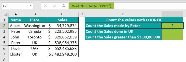
Step 4: Enter the formula, =COUNTIF(B2:B7,“UK”) in cell F3.

Step 5: Press the “Enter” key. The output is 2, as shown below, i.e., there are 2 sales in the UK.
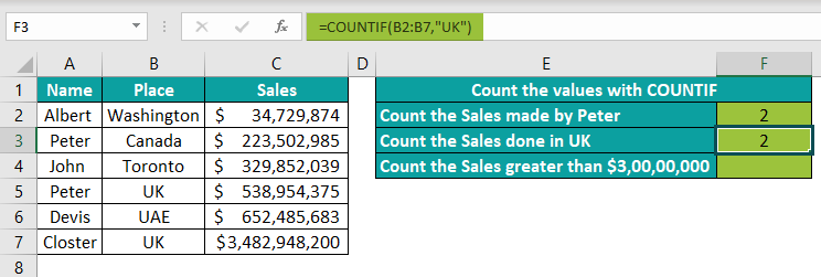
Step 6: Finally, enter the formula, =COUNTIF(C2:C7,“>30000000”) in cell F4.

Step 7: Press the “Enter” key. The output is 6, as shown below, i.e., there are 6 sales greater than $30,000,000.

- Therefore, the COUNTIF function in Excel counts all the Sales made by Peter, the Sales done in the UK, and the Sales greater than $3,00,00,000 as per the respective conditions.
Important Things To Note
- There are five variants of the COUNT function group, namely, COUNT function, COUNTA function, COUNTIF, COUNTIFS, and COUNTBLANK.
- The COUNTIF Excel Function returns the #VALUE! Error if the text in the criteria has more than 255 characters in length.
- The second argument of the function is “Criteria”, which is not case sensitive.

Frequently Asked Questions (FAQs)
The COUNTIF Excel Function is a member in the COUNT function list, like the COUNTA and COUNTBLANK functions. It is a pre-defined function in Excel that counts all the cells in the cell range as specified by the conditions.
The COUNTIF formula in Excel is,
=COUNTIF(range,criteria)
We use the COUNTIF Excel Function in large datasets to count the duplicate values and also for data with logical operators (>,<,< >,=), as the function supports logical operators.
The step-by-step procedure to find the COUNTIF Excel Function is,
1. Select the “Formulas” tab.
2. Go to the “Function Library” group.
3. Click on the “More Functions” option.
4. Click on the “Statistical” option.
5. Select the “COUNTIF” option.
6. The “Function Arguments” window pops up.
7. Enter the values in the “Range” and “Criteria” fields.
8. Click OK.
Download Template
📥Download the ready-to-use Excel template to practice this tutorial yourself.
COUNTIF Excel functionRecommended Articles
This has been a guide to COUNTIF Excel Function. Here we learn the COUNTIF Function, formula, examples of different scenarios & downloadable excel template. You can learn more from the following articles –

Leave a Reply