Strikethrough In Excel

What Is Strikethrough In Excel?

The Strikethrough in Excel is a font feature where a horizontal line appears striking through the value displayed in the cell. It appears at the center of the cell. Using Strikethrough in Excel in a cell indicates that the text or a character with a strike can be ignored or removed.

Top Six Methods To Strikethrough In Excel

We will use Strikethrough in Excel in six different ways, namely,

1. Using Excel Shortcut Key.
2. Using Format Cell Options.
3. Using from Quick Access Toolbar.
4. Using it from Excel Ribbon.
5. Using Dynamic Conditional Formatting.
6. Using VBA.

#1 – Using Excel Shortcut Key

We will understand Strikethrough text Excel using the Excel shortcut keys [Ctrl+5].

In the table, the data is as follows:

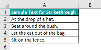
• Column A contains the Sample Text for Strikethrough.

The steps to Strikethrough in Excel using the Excel shortcut keys are,

Step 1: Select the cells A3 and A4.

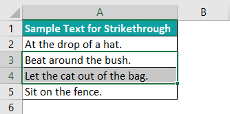
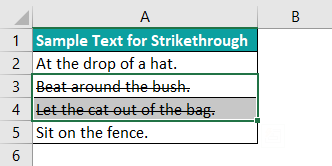
Step 2: Press the shortcut key CTRL+5. The output is shown below.

#2 – Using Format Cell Options

We will understand Strikethrough text Excel using the Format cells options.

In the table, the data is as follows:

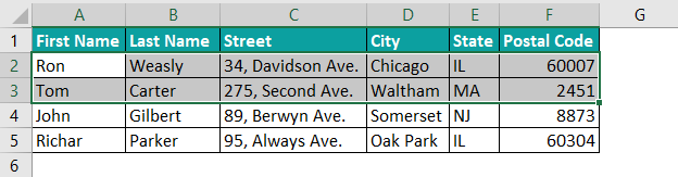
• Column A contains the First Name.
• Column B contains the Last Name.
• Column C contains the Street.
• Column D contains the City.
• Column E contains the State.
• Column F contains the Postal Code.

The steps to Strikethrough in Excel using the Format Cells option are,

Step 1: Select the cell range A2:F3.

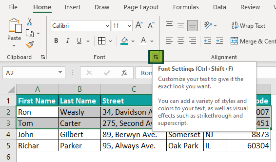
Step 2: Select the “Home” tab > go to the “Font” group > click on the “Font Settings” launcher. [Alternatively, we can use the shortcut keys Ctrl+Shift+F].

Step 3: Now, the “Format Cells” window opens. Under the “Font” menu, check/tick the “Strikethrough” checkbox in the “Effects” option.

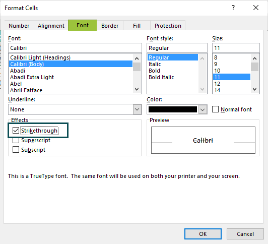
Step 4: Click on “OK”. The output is shown below.

#3 – Using From Quick Access Toolbar

We will understand Strikethrough text Excel using the Quick Access Toolbar.

In the table, the data is as follows:

• Column A contains the First Name.
• Column B contains the Last Name.
• Column C contains the Full Name.

The steps to Strikethrough in Excel using the Quick Access Toolbar are,

Step 1: Select the “File” tab > go to the “More…” options from the menu > select the “Options” as shown below.

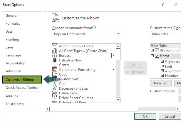
Step 2: The “Excel Options” window opens. Now, select the “Customize Ribbon” option on the left side menu of the “Excel Options” window, as shown below.

Step 3: On the right side, in the “Main tabs” window, open the “Home” option and then click on the “New Group” button below the “Main tabs” window. Immediately, a “New Group(Custom)” is created inside the “Home” option.

Step 4: Click on the “Rename” button below the “Main tabs” window. When the “Rename” window opens, then, in the “Display name:” field, type “My Formats”, as shown below.

Step 5: On the left of the “Main Tabs”, click on the “Choose Commands from” drop-down and then select the “Commands Not in the Ribbon” option.

Step 6: Once we select the “Commands Not in the Ribbon” option in the window below, scroll down to “Strikethrough” > click on the “Add” button on the right > click on “OK”. Immediately, the “Strikethrough” command is added to the “My Formats” group, as shown below.

On the “Home” tab, the “My Formats” group is created, with the “Strikethrough” option, as shown below.

Step 7: Finally, select cell A2, go to the “Home” tab > go to the “My Formats” group > click on the “Strikethrough” option. The output is shown below.

#4 – Using It From Excel Ribbon

We will understand Strikethrough text Excel using it from the Excel ribbon options.

In the table, the data is as follows:

• Column A contains the Emp. ID.
• Column B contains the Emp. Name.
• Column C contains the Annual Salary.

The steps to Strikethrough in Excel using the Excel Ribbon are,

Step 1: Select the “File” tab > go to the “More…” options from the menu > select the “Options” as shown below.

Step 2: The “Excel Options” window opens. Now, select the “Customize Ribbon” option on the left side menu of the “Excel Options” window, as shown below.

Step 3: On the right side, click on the “New Tab” button below the “Main tabs” window. Immediately, a “New Tab(Custom)” option appears under the “Home” option.

Step 4: Click on the “Rename” button below the “Main tabs” window, and a “Rename” window pops up. In the “Display name:” field, type “Strikethrough”, as shown below.

Step 5: On the left of the “Main Tabs”, click on the “Choose Commands from” drop-down and then select the “Commands Not in the Ribbon” option.

Step 6: Once we select the “Commands Not in the Ribbon” option in the window below, scroll down to “Strikethrough” > click on the “Add” button on the right > click on “OK”. Immediately, the “Strikethrough” tab is added to the ribbon, as shown below.

On the ribbon, we will now see a “New Tab” tab with the “Strikethrough” group, as shown below.

Step 7: Finally, select cell B2, go to the “New Tab” tab > go to the “Strikethrough” group > click on the “Strikethrough” option. The output is shown below.

#5 – Using Dynamic Conditional Formatting

We will understand Strikethrough text Excel using the Dynamic Conditional Formatting.

In the table, the Pokémon data is as follows:

• Column A contains the Name.
• Column B contains the Type.

The steps to Strikethrough in Excel using the Dynamic Conditional Formatting are,

Step 1: Select the cell range, A2:A5.

Step 2: Select the “Home” tab > go to the “Styles” group > click on the “Conditional Formatting” drop-down > select the “New Rule…” option, as shown below.

The “New Formatting Rule” window opens, as shown below.

Step 3: Select the “Use a formula to determine which cells to format” option from the “Select a Rule Type:” window.

Step 4: In the “Edit the Rule Description:” inside the “Format values where this formula is true:” field, type the formula, =B2=“Fighter” and then click on the “Format” button.

Step 5: The “Format Cells” window opens, now check/tick the “Strikethrough” option in the “Effects” window.

Step 6: Finally, click on “OK”, the “Format Cells” window closes, and once again click on “OK”, the “New Formatting Rule” window closes. The output is shown below. [In Column B, when the “Type” is “Fighter”, then the respective Pokémon “Name” in Column A is crossed, according to the “Conditional Formatting”]

#6 – Using VBA

We will understand Strikethrough text Excel using VBA.

In the table, the data is as follows:

• Column A contains the text “Sample Text for Strikethrough”.

The steps to Strikethrough in Excel using the VBA are,

Step 1: Open an Excel workbook. By default, we will see the worksheet “Sheet1”. Select cell A1 and type “Sample text for Strikethrough”.

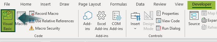
Step 2: Next, select the “Developer” tab > go to the “Code” group > click on the “Visual Basic” option, as shown below.

Step 3: The “Microsoft Visual Basic for Applications” window pops up on the left pane, then double-click on “Sheet1(Sheet1)”. The “Sheet1 (Code)” window opens, as shown below.

Step 3: In the “Sheet1 (Code)” window, type the following code,

Sub font()

Range(“A1”) = “Sample Text for Strikethrough”

Range(“A1”).font.Strikethrough = True

End Sub

Step 4: To run or execute the code, select the “Run” tab from the menu > click on the “Run Sub/UserForm” option.

The output is shown below. [The moment we execute the code, a strike appears on the text in the cell].

How To Remove Strikethrough In Excel?

We can Remove Strikethrough in Excel using the Strikethrough shortcut Excel keys, “Ctrl+5”.

In the table, the data is as follows:

• Column A contains the text “Sample Text for Strikethrough”.

The steps to Remove Strikethrough in Excel using the Strikethrough shortcut Excel keys are,

Step 1: Select cell A1 and press the shortcut keys Ctrl+5. A strike appears on the text in the cell.

Step 2: Select cell A1 again and press the Strikethrough shortcut Excel keys Ctrl+5. The output is shown below. [The strike disappears, and the text appears as before].

Important Things To Note

• In a cell, we can apply the Strikethrough in Excel, even to just an alphabet or a character. For example, My Name is John.
• When we apply Strikethrough in Excel to any cell, the cell’s value does not change, and only the horizontal line appears. So, for example, “TEXT” and “TEXT” are equal.
• We can apply Strikethrough in Excel by creating a “New Rule” using “Conditional Formatting”.

Frequently Asked Questions

Download Template

This article must help understand Strikethrough in Excel with its formulas and examples. You can download the template here to use it instantly.

Recommended Articles

This has been a guide to Strikethrough in Excel. Here we discuss top six methods to Strikethrough and how to remove it with examples and downloadable excel template. You can learn more from the following articles –

• Basic Excel Formulas
• FILTER In Excel
• Errors In Excel