
What Is Conditional Formatting In Excel?
Conditional Formatting is a dynamic process of formatting the cell or range of cells based on the conditions of the users. It highlights the cells, applies font formatting, creates in-cell bar charts, increases or decreases icons, highlights duplicate values, highlights one cell based on the value in the other cell, top 10 and bottom 10 values, creates heat maps, etc.
For instance, the following table shows the regional sales data of salespersons.
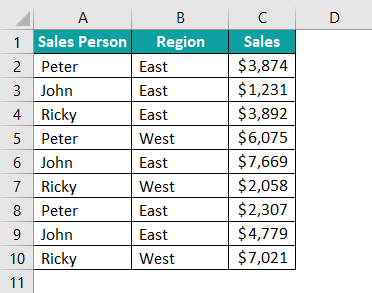
Assume we need to highlight the cells with ‘West’ under the Region column, then we can use conditional formatting to highlight those cells.
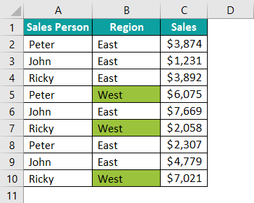
Whenever values in the range B2:B10 change to West, conditional formatting automatically highlights those cells.
Use this Conditional Formatting in Excel Template to follow along with the examples in this article.
Download Excel TemplateKey Takeaways
- Conditional formatting in Excel is used to format cells based on the criteria given by users.
- We can apply conditional formatting only for the logical tests.
- We can create a new rule and write it to be validated and apply conditional formatting if the rule is TRUE.
- Also, users can apply multiple conditional formatting rules for even a single cell in Excel.
- Similarly, it is possible to apply conditional formatting for multiple cells based on one cell value.
How To Access Conditional Formatting?
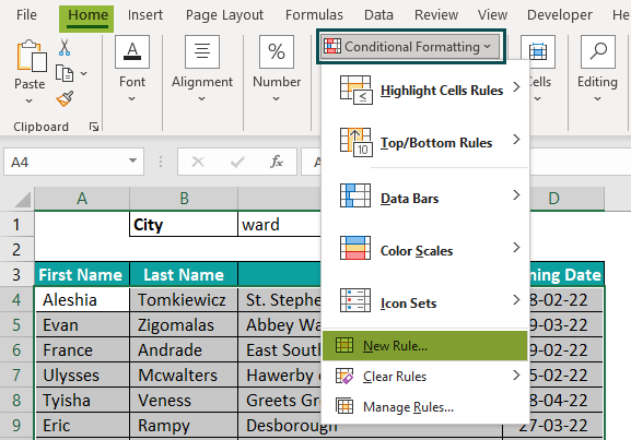
Conditional Formatting is a built-in tool in Excel; we can access this feature from the Home tab in Excel.
Go to the Home tab, and under the Styles category, we have an option called Conditional Formatting.

Click on the drop-down list of conditional formatting to see variety of conditional formatting options.
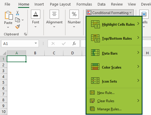
Based on the requirement, we can choose the appropriate conditional formatting.
How To Use Conditional Formatting? (With Steps)
Let us understand how to use conditional formatting with a few examples.
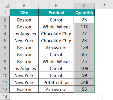
For instance, we have the following city-wise sales for different products.
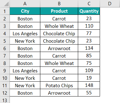
Assume we need to highlight the cells where the quantity is more than 100. Following are the steps to apply conditional formatting.
Step 1: Select the cells in the range C2:C12.
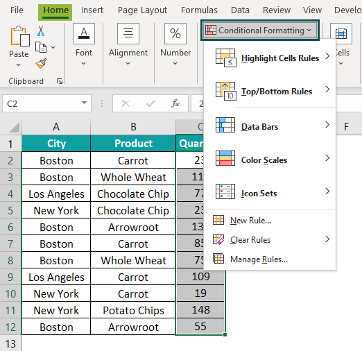
Step 2: Go to the Home tab and click on the drop-down list of Conditional Formatting.
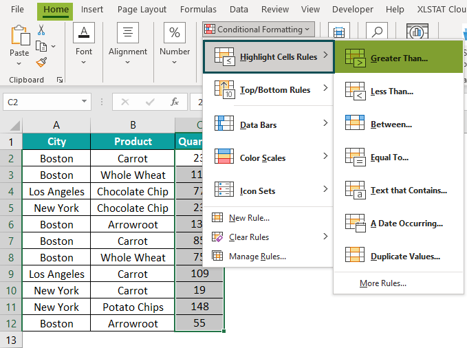
Step 3: Hover the mouse on Highlight Cells Rules, and it will display various options. Click on the Greater Than… option.
Step 4: The Greater than window pops up. In the Format cells that are GREATER THAN: box, enter the value as 100.
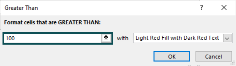
Step 5: Next, choose the formatting option from the drop-down list.
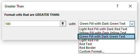
Step 6: After choosing the appropriate formatting option, click OK.
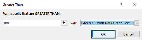
After clicking OK, it will highlight the cells with a value of >=100.
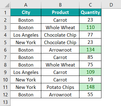
As we can see in the above image, cells that have a value >=100 are colored green with green font.
Similarly, if we want to highlight the cells with a value <100, then choose Less Than… option.

Then, in the Less than window, enter the value as 100 and choose the formatting as Light Red Fill with Dark Red Text.

Click on OK. It will apply the formatting for all cells with a value of <100.
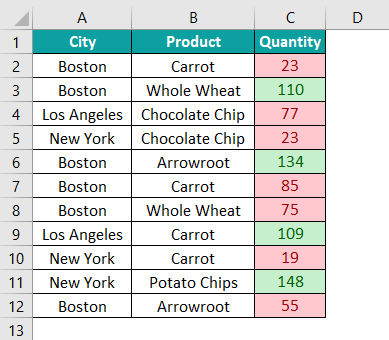
Now all the cells with a value of >=100 are formatted with Light Green Fill with Dark Green Text, and cells with a value of <100 are formatted with Light Red Fill with Dark Red Text.
Advanced Conditional Formatting Usage
Example 1 – Create New Rules
The conditional formatting feature comes with various built-in options. However, users can use the New Rule feature if they want to apply their rules to conditional formatting.
For instance, we have the following state-wise and product category-wise sales units’ data in an Excel spreadsheet.
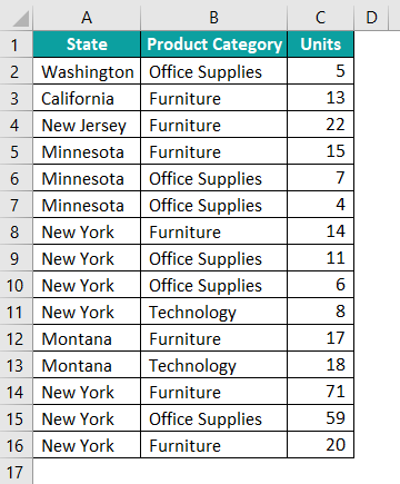
Here we need to highlight the rows where the units sold are >=15 but also for the state New York and the category Furniture.
In this example, we have the following 3 conditions to apply formatting i.e.
Units >=15
State = New York
Product Category = Furniture.
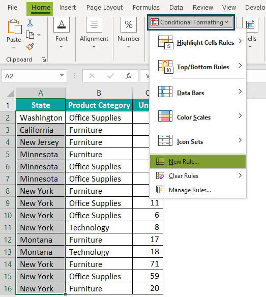
Step 1: To start with, select the entire data range from A2:A16.
Step 2: Go to the Home tab.
Step 3: Next, click on the drop-down list of Conditional Formatting and then, choose New Rule.
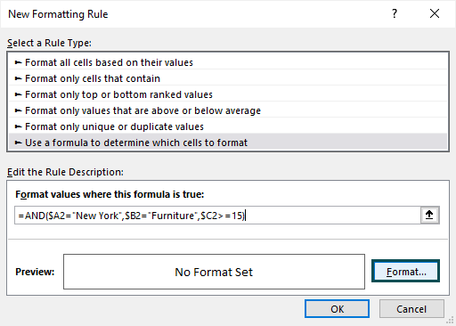
Step 4: The New Formatting Rule window pops up. Click on Use a formula to determine which cells to format option.
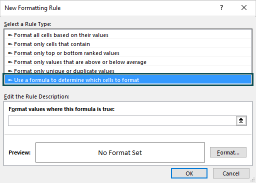
Step 5: In the Format values where this formula is true: box, we need to type a formula to determine the cells which satisfy the conditions.
Then, apply the following AND function.
=AND($A2=”New York”,$B2=”Furniture”,$C2>=15)
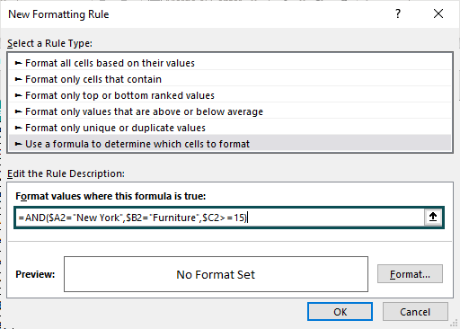
AND function here checks for the New York state in column A, Furniture category in column B, and checks which cell has the number of units >=15.
When all the above 3 conditions are met, the AND Excel function will return TRUE.
Step 6: Now, click on the Format… option.
Step 7: The Format Cells window opens up. Choose the Fill option and select the fill color (as required).
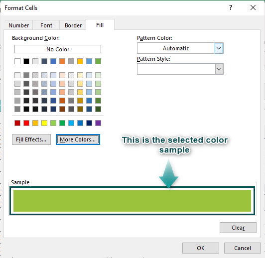
Step 8: Click on OK. It will revert to a conditional formatting window.

Step 9: Click on OK. Now we can see the conditional formatting applied to the cells wherever the applied conditions are met.
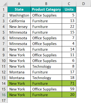
In rows 14 & 16, we have a state, product and units sold categories.
Example 2 – Based On Cell Value
The above example taught us how to highlight cells with a pre-defined set of values. But if the user wants to highlight any other value cells, they need to apply another conditional formatting or edit the existing conditional formatting rule.
Since it is a tedious and manual process, we can give users the option of entering the values they want to highlight, and conditional formatting will do the job for them.
For instance, we have the following employee name database in an Excel spreadsheet.

The objective here is to allow the user to enter the city name in cell C1, and conditional formatting should highlight the entire row with the city typed in cell C1.
Step 1: Select the entire data range from A2:A16.
Step 2: Go to the Home tab.
Step 3: Click on the drop-down list of Conditional Formatting and choose New Rule… option.
Step 4: The New Formatting Rule window pops up. Click on Use a formula to determine which cells to format option.
Step 5: In the formula box, write the following conditional formatting in excel formula.
=AND($C$1<>””,ISNUMBER(SEARCH($C$1,$C4)))

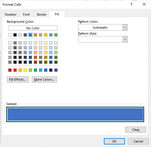
Step 6: Click on the Format tab and choose the fill color we want.
Click OK in the following two tabs. Then, we will be back to the spreadsheet.
Now, enter the word Hill in cell C1 and hit the Enter key.
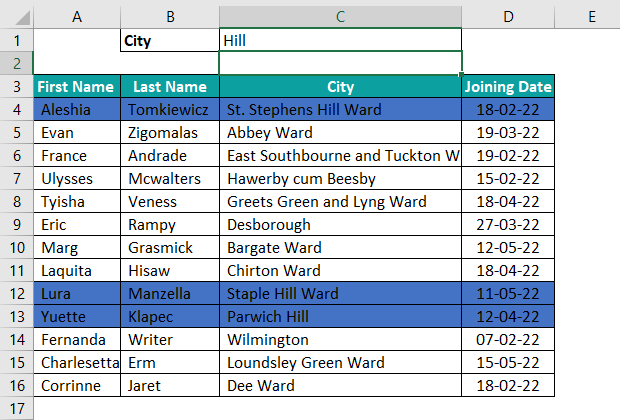
When we type the city’s name, Excel highlights the rows with the word Hill using conditional formatting in excel.
Similarly, type the word Ward and hit the Enter key.
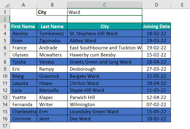
Now, all the cities which have the word Ward are highlighted by conditional formatting.
Explanation of the Formula: =AND($C$1<>””,ISNUMBER(SEARCH($C$1,$C4)))
First, AND function will check whether the value in cell C1 is blank.
Then SEARCH excel function will find if the typed city name in cell C1 is part of the city name in column B or not. If the typed word is part of any city name, then the SEARCH function will return the starting number of that word in the city names.
Then, the ISNUMBER excel function would return TRUE if the value provided by the SEARCH function is a numerical value.
Then, AND function will evaluate both the conditions and return the result as TRUE, and the respective rows will be highlighted with conditional formatting in excel.
Example – 3 – Multiple Conditional Formatting Rules In One Cell/Table
It is possible to apply multiple conditional formatting rules for one single cell. For instance, assume there is a score in one of the cells, and we want to highlight the cell with red if the score is <3. If we want to highlight the cell with yellow if the score is between 4 to 8 and highlight the cell with green if the score is >=8.
We have the following student scores in an Excel spreadsheet.

Now we need to highlight the score cells based on the following criteria.
- If the score cell is blank, we need to highlight those cells in Grey.
- Similarly, if the score cell is >0, the cells are highlighted in red.
- If the score cell is >50, we need to highlight those cells in Yellow.
- Likewise, if the score cell is >90, we need to highlight those cells in Green.
Step 1: Select the entire data range from C2:C11.

Step 2: Go to the Home tab.
Step 3: Click on the drop-down list of Conditional Formatting and choose New Rule… option.
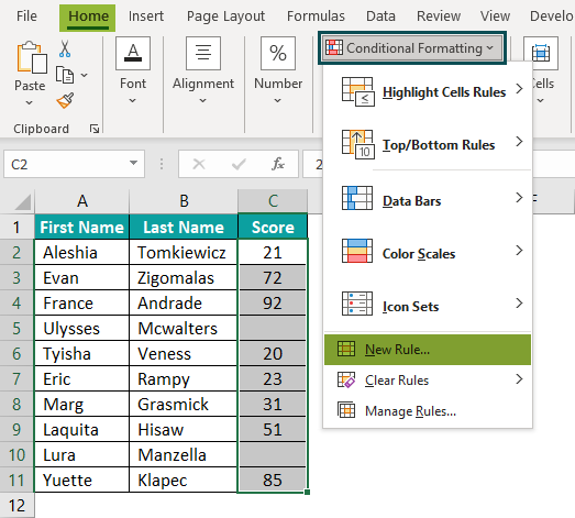
Step 4: The window, New Formatting Rule appears. Click on Use a formula to determine which cells to format option.
Step 5: Type =ISBLANK(C2) as the formula.

Step 6: Click on the Format button and choose the fill color as Grey.

Click OK.
Then, we will be back to the New Formatting Rule window.

Step 7: Click on OK again. Now, we can see that all the blank cells are highlighted in grey.

Step 8: Now, we need to apply 3 other rules. Selecting the range of cells from C2:C11, go to the Conditional Formatting drop-down and click on the Manage Rules… option.

Step 9: The Conditional Formatting Rules Manager window opens. Now, click on the New Rule… button.

Step 10: The New Formatting Rule window appears. Click on the Use a formula to determine which cells to format option.
Step 11: In the formula box, write the following conditional formatting in excel formula.
=C2>0.

Step 12: Click on the Format tab, and choose the fill color as Red.

Step 13: Click on OK. We can see that the Conditional Formatting Rules Manager window appears again.

Step 14: Now, repeat the same step for scores >=50 and >=90. We will end up with 4 different formatting rules for a single cell.

Step 15: Click on OK. We should be able to see the formatting for all the score cells.

All the score cells are shown in red because we have applied conditional formatting in excel. If we look back at the previous window, the first formatting condition is >0; then it should be filled with red. Hence, the formatting rule satisfied the first logic and applied red fills for all the cells.
As per our formatting rule highest criteria, i.e., cell value >90, should come first; select this rule and use the Move Up button.

Arrange the rules shown in the above image.
Green first, Yellow Second, and Red at last.
Note: Order of rule also matters in conditional formatting. It is why we should sort the formatting rules in order.
After arranging the formatting rules in the above order, click OK. Now, the formatting will work fine.

Like this, we can apply multiple formatting rules for one cell.
How To Edit Conditional Formatting Rules?
After applying conditional formatting, we can edit and change the rules per our needs.
For instance, in the following image, we have a few numbers, and we have already applied the conditional formatting rule to highlight the number >40.

Assuming we need to change the formatting rule from >40 to >45.
So, in this case, select the range of cells from A2:A11.

Go to the Home tab and click on the Conditional Formatting drop-down list. Then, click on Manage Rules… option.

Now, the Conditional Formatting Rules Manager window opens. Select the rule and click on the Edit Rule… option.

When we click on the Edit Rule option, it will display the Edit Formatting Rule window. In this window, we can change the rule.

Note: Not only the rules but also, we can change the formatting styles as well by clicking on the Format button.
Click on OK, and now the formatting will highlight the cells with a value >45.

Copy Conditional Formatting Rules
By Using Paste Special: We can also copy conditional formatting rules from one cell, worksheet, and workbook to another.
For instance, in the following image, we have a set of numbers and applied conditional formatting to highlight the cells with values between 500 to 600.

Now we have another set of values next to it.

We need to apply the same conditional formatting as we have applied for Set 1 for this set too.
Step 1: Select and copy a cell in Set 1.
Step 2: After copying the cell in Set 1, choose the Set 2 range of cells from C2:C11.
Step 3: Right-click on the selection and click on Paste Special… option.

Step 4: The Paste Special window opens up. Choose the Formats option in this window.

Step 5: Click OK to apply formatting from Set 1 to Set 2..

As shown in the above image, we have numbers highlighted between 500 to 600.
By Using Format Painter: We can also copy conditional formatting using the format painter option.
Select any cell in Set 1 numbers and click on the Format Painter.

After selecting Format Painter, it will activate the format painter tool. Now, select all the cells of Set 2 values, and immediately conditional formatting will be applied to Set 2 values.

Important Things To Note
- Conditional Formatting is volatile and will impact the workbook’s performance. Excel workbook tends to slow down.
- Conditional Formatting in Excel accepts only logical formula which gives either TRUE or FALSE results.
- When we copy the cell with conditional formatting, it will also copy the formatting rule.
- When multiple rules are applied to a single cell, we need to choose the order of rules to make it properly.
- We can use the pre-defined rules to format based on rules. For example, highlight the top 10 or bottom 10 values.
Frequently Asked Questions (FAQs)
For instance, we have the following city names in an Excel spreadsheet.
We need to highlight the cells with the value ‘London’ by applying conditional formatting.
Step 1: Select the entire data range from A2:A16.
Step 2: Go to the Home tab.
Step 3: Then, click on the drop-down list of Conditional Formatting and choose New Rule.
Step 4: The New Formatting Rule window pops up. Click on the Use a formula to determine which cells to format option.
Step 5: In the Format values where this formula is true: box, enter the following formula.
Step 6: In the above window, click the Format option and apply the formatting as needed.
Step 7: Click on OK. Then, we should see the highlighted cell with the value ‘London’.
Using conditional formatting in excel, we can format the cells based on the set of conditions. By applying conditional formatting, we can make the formatting dynamic. Also, whenever changes are made in data formatting, they will be applied dynamically.
Go to the Home tab and click on the Conditional Formatting drop-down list under the Styles category.
Based on the requirement, we can choose the appropriate conditional formatting.
After applying conditional formatting in excel, protect the worksheet by unchecking all the formatting options.
Use this Conditional Formatting in Excel Template to follow along with the examples in this article.
Download Excel Template