ISNUMBER in Excel

What Is ISNUMBER Function In Excel?

The ISNUMBER in Excel detects the numeric value cells and returns the answer in Boolean. If the cells are numeric values, we get the result as TRUE; else, we will get the result as FALSE. The ISNUMBER Function detects a cell that contains a number starting from 0 to any digit. The function returns TRUE if there is a numerical value, or else the function will return FALSE.

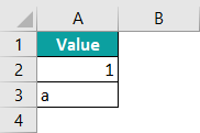
For example, the below table shows the numeric value in cell A2 and the alphabetical value in cell A3. Let us apply ISNUMBER in excel formula to obtain the results.

The steps used to check ISNUMBER in Excel are as follows:

Step 1: First, select the cell to display the output. In this example, we select cell B2.

Step 2: Next, enter the ISNUMBER formula in cell B2. So, the complete formula is =ISNUMBER(A2).

Step 3: Then, press Enter key.

Clearly, we can see that the result is returned as TRUE for numeric value ‘1’ and

FALSE for alphabetic value ‘a’.

Likewise, we can use the ISNUMBER in excel to detect numerical values.

What Is ISNUMBER Function In Excel?

The ISNUMBER function returns a Boolean value, i.e., TRUE or FALSE. It is used to find cells with numeric values on the worksheet.
This function is very helpful in detecting numeric values in large data.
The function returns FALSE when the value is non-numeric, i.e., text or other special characters.
Similarly, the function returns TRUE when the value is numeric.
ISNUMBER function never returns an error value like #NAME!, #N/A! etc.
The ISNUMBER function is one of the functions categorized under the Information group.

ISNUMBER() Excel Formula

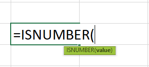
The syntax of the ISNUMBER in Excel is –

where,

value: It is the mandatory argument and denotes the targeted cell we want to test.

Excel VBA – All in One Courses Bundle (35+ Hours of Video Tutorials)

If you want to learn Excel and VBA professionally, then Excel VBA All in One Courses Bundle (35+ hours) is the perfect solution. Whether you’re a beginner or an experienced user, this bundle covers it all – from Basic Excel to Advanced Excel, Macros, Power Query, and VBA.

Start Learning Now

How To Use ISNUMBER Excel Function (With Steps)

Access ISNUMBER function from the Excel ribbon.

To begin with, choose an empty cell to display the output.
Go to the Formulas tab and select More Functions from the drop-down menu.
Select Information from the list of options.
Scroll down and click on the ISNUMBER
The Function Arguments window pops up.
Based on the number of arguments, enter the value in the Value
Select OK.

2. Enter the worksheet manually

Select an empty cell to display the output.
Type =ISNUMBER( in the selected cell.

Alternatively, type =I and double-click on the ISNUMBER function from the list of suggestions shown by Excel.

Enter the arguments as cell references or direct values.
Close the parenthesis and press Enter

Basic Example

The below table shows the general data as values in column A. But, first, let us understand how to use ISNUMBER in Excel using the following steps.

The steps to detect the numeric values using ISNUMBER in Excel are as follows:

Step 1: First, we should select the column to display the result.

For our example, let us select column B.

Step 2: Enter the ISNUMBER formula in cell B2. Since we need to detect if the value in cell A2 is numerical or not, A2 is the argument used in this function.

So, the complete formula is =ISNUMBER(A2).

Step 3: Press Enter key. We can see that the function has returned the result as TRUE in cell A2, as shown in the following image.

Step 4: Insert the function in the other cells or use the AutoFill option. Let us use the AutoFill option and drag the cursor to cell B5.

We can see that the function has returned FALSE in all the cells except in cell A2. The results clearly show that the table has non-numerical values in the range A3:A5.

And A2 is a numeric value cell.

Similarly, we can detect numerical values using ISNUMBER in excel.

Examples

Example 1 – ISNUMBER With Cell Reference In Excel

The below table shows mixed values in column A. Let us detect numerical values using the ISNUMBER function with Cell Reference in Excel.

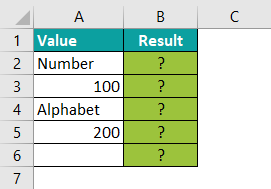
The steps used to detect the numeric value using ISNUMBER in Excel are as follows:

Step 1: To begin with, select the column to display the result. In this case, let us select column B.

Step 2: Next, enter the ISNUMBER formula in cell B2.

The complete formula is =ISNUMBER(A2).

Step 3: Then, press Enter key.

We can see that the function has returned the result as FALSE in cell A2, as shown in the following image.

Step 4: We can either insert the ISNUMBER in Excel formula is each cell or use the AutoFill option.

Let us use the AutoFill option. First, drag the cursor to cell B6.

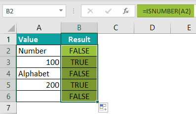
We can see that the function has returned TRUE in cells B3 and B5. It indicates that cells A3 and A5 have numeric values.

Similarly, the function has returned FALSE in cells B2, B4, and B6. It indicates that cells A2, A4, and A6 have non-numeric values.

Likewise, we can detect numerical values using ISNUMBER in excel formula.

Example 2 – ISNUMBER With Data Validation

The following table shows mixed values in column A. Now, let us understand how to detect numerical values using ISNUMBER in Excel with Data Validation.

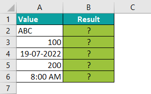
The steps to detect numeric values using IF and ISNUMBER in Excel are as follows:

Step 1: Select the cell to display the result. In this case, we have selected cell B2.

Step 2: Enter the ISNUMBER in excel formula along with the IF formula.

So, the complete formula is =IF(ISNUMBER(A2),“Numeric”,“Non-Numeric”).

Step 3: Press Enter key.

We can see that the function has returned Non-Numeric in cell B2, as shown in the following image. It is because it indicates that cell A2 contains an alphabetic value.

Step 4: We can insert the function in all the cells or use the AutoFill option to obtain the result in other cells.

Let us use the AutoFill option. So, drag the cursor to cell B6.

We can clearly see that the function has returned Non-Numeric in cell B2. It is because it indicates that cell A2 has an alphabetic value.

Similarly, the function has returned Numeric in cells B3, B4, B5, and B6, indicating that cells A3, A4, A5, and A6 have numeric values.

Similarly, using IF and ISNUMBER in Excel, we can detect numeric values.

Example 3 – Combining ISNUMBER And SEARCH Functions To Find A Substring

The SEARCH Function in Excel returns the position or index value of a specified substring within a text string. The function is part of the TEXT functions group. The SEARCH function can also search text and supports the use of wild cards.

The formula of the SEARCH function in Excel is

=SEARCH(find_text,within_text,[start_num])

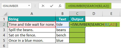
The following table shows the text string and the searched text in columns A and B, respectively. But, first, let us understand how to search for numeric values using the SEARCH function and ISNUMBER in Excel.

The steps used to detect the cells with numeric values using ISNUMBER in Excel are as follows:

Step 1: Select the cell to display the output. In this example, let us select cell C2.

Step 2: Enter the ISNUMBER formula with the SEARCH formula in cell C2.

So, the complete formula is =ISNUMBER(SEARCH(B2,A2)).

Step 4: Press Enter key.

We can see that the function has returned TRUE in cell C2, as shown in the following image. Also, the SEARCH function in cell A2 returns the index value as ‘10’, which is the numeric value.

Step 5: Now, using the AutoFill option, drag the cursor to cell C5.

We can see that the SEARCH function has returned the index value as ‘10’ in cell A2, which is the numeric value. So, the output is TRUE.

Similarly, the SEARCH function has returned the index value as ‘11’ in cell A3, which is the numeric value. So, the output is TRUE.

The SEARCH function in cell A4 has returned the #VALUE! error, which is the non-numeric value. So, the output is FALSE.

Similarly, the SEARCH function has returned the index value as ‘11’ in cell A5, which is the numeric value. So, the output is TRUE.

Example 4 – ISNUMBER With Conditional Formatting In Excel

The below table shows values in the range A2:C4. We need to use the following steps to search numeric values using the ISNUMBER function with Conditional Formatting in Excel.

The steps to detect the numeric values using ISNUMBER in Excel are as follows:

Step 1: Select the table array.

Step 2: Go to the Home tab.

Step 3: Select the Conditional Formatting option from the Style group.

Step 4: Click on the New Rule… option.

Step 5: The window, New Formatting Rule, pops up.

Step 6: Select the Use a formula to determine which cells to format option.

Step 7: Enter the formula in the Format values where this formula is true: box.

So, the formula is =ISNUMBER(A2:C4).

Step 8: Click the Format… button to set the color of the blank cells.

Step 9: The Format Cells window opens.

Step 10: Under the Fill menu, select the Background color.

Step 11: Click OK.

Step 12: The Format Cells window gets closed.

Step 13: Click OK in the New Formatting Rule window.

Step 14: The numeric values will be highlighted in yellow, as shown in the below image.

Likewise, we can use the ISNUMBER function with Conditional Formatting in Excel.

ISNUMBER Excel Function Not Working

We know that the ISNUMBER in Excel returns a Boolean value, true or false, i.e., TRUE for numeric values and FALSE for non-numeric values. The ISNUMBER function may not work in Excel because of extra spaces between formulas; In simple words, when we enter incorrect formulas, the function does not work correctly.

Frequently Asked Questions

How to use ISNUMBER in Excel?

Let us understand the use of ISNUMBER with an example.

The below table shows mixed values in column A. Now, we need to detect the cells with numeric values check ISNUMBER in Excel function.

FAQ 1

The steps used to check ISNUMBER in Excel are as follows:

Step 1: First, select a cell to display the output. In this example, let us select cell B2.

Step 2: Next, enter the formula in cell B2.

So, the complete formula is =ISNUMBER(A2).

Step 3: Then, press Enter key.

We can see that the function has returned TRUE for numeric value ‘100’ and FALSE for all other values (alphabetic and special characters).

FAQ 1.1

Likewise, we can use ISNUMBER in Excel function to detect numerical values.

What is the use of ISNUMBER in Excel?

The ISNUMBER in Excel detects whether a cell contains a number or not. The function returns True if the value is numeric; if not, it returns False.

How do ISNUMBER and ISTEXT functions differ?

ISNUMBER in Excel
– The function checks whether a value in a cell or a value from another formula is a number.
– The output of ISNUMBER is either TRUE or FALSE

ISTEXT in Excel

– The function checks whether a value is a text or not.
– The output of ISTEXT is also either TRUE or FALSE

Therefore, using both functions, we can find if a value in a cell is a numeric value or text value.

Download Template

This article must help understand ISNUMBER in Excel with its formula and examples. You can download the template here to use it instantly.

ISNUMBER in Excel Download

ISNUMBER in Excel