
What Is SUBTOTAL function In Excel?
The SUBTOTAL function in Excel performs the arithmetic operations or basic Excel functions such as average, count, sum, max, min, product, etc. Primarily, the SUBTOTAL function is designed for vertical cell ranges and not for horizontal cell ranges. Therefore, we can apply the SUBTOTAL function only for a column or columns and not for rows.
This SUBTOTAL function is an inbuilt function in Excel that allows the user to insert it as a function from the “Function Library” or enter the “SUBTOTAL formula” directly in the cell.
Use this SUBTOTAL Function In Excel Template to follow along with the examples in this article.
Download Excel TemplateKey Takeaways
- The SUBTOTAL function performs a specific calculation on numeric values when we insert the function number according to the function_num list.
- We can insert multiple SUBTOTAL formulas in a vertical range column or columns and break the data into various categories. However, the SUBTOTAL function does not work on a horizontal range of cells or rows.
- A SUBTOTAL function will give the output for numeric values.
SUBTOTAL() Excel formula
The syntax of the SUBTOTAL in Excel is,

The arguments of the SUBTOTAL in Excel are,
- function_num – It describes which function to use in the SUBTOTAL function. It is a mandatory argument.
- ref1 – It is the Excel cell reference of the SUBTOTAL function. It is a mandatory argument.
Operations Performed By The SUBTOTAL Function (function_num)
The SUBTOTAL function executes an arithmetic operation depending on the value provided in the “function_num” argument. The operations executed by the SUBTOTAL function are as follows:
| Function | function_num (Hidden values Included) | function_num (Hidden values Excluded) |
|---|---|---|
| AVERAGE | 1 | 101 |
| COUNT | 2 | 102 |
| COUNTA | 3 | 103 |
| MAX | 4 | 104 |
| MIN | 5 | 105 |
| PRODUCT | 6 | 106 |
| STDEV.S | 7 | 107 |
| STDEV.P | 8 | 108 |
| SUM | 9 | 109 |
| VAR.S | 10 | 110 |
| VAR.P | 11 | 111 |
The function_num argument can use any values from the “hidden values included” or “hidden values excluded” list.
How To Use SUBTOTAL() In Excel?
We can use the SUBTOTAL() In Excel using two methods,
Method 1 – Access from the Excel ribbon,
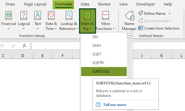
Select the “Formulas” tab > go to the “Function Library” group > click on the “Math & Trig” option drop-down > select the “SUBTOTAL” option, as shown below.
The “Function Argument” window pops up, as shown below,

Then, enter the arguments in the “Function_num” and the “Ref1” fields and click on “OK”.
Method 2 – Enter the SUBTOTAL formula in the worksheet manually,
- Select an empty cell.
- Type =SUBTOTAL( in the selected cell. [Alternatively, type =S and double-click on the SUBTOTAL function from the list of suggestions shown by Excel].
- Enter the arguments as cell references or direct values.
- Close the parenthesis and press the “Enter” key.
We will use the SUBTOTAL function using the COUNT Excel function number in Excel.
The data is as follows,
- Column A contains the Value.
The steps to demonstrate the SUBTOTAL function are as follows:
Step 1: Select cell A6 for the output.

Step 2: Enter the formula, =SUBTOTAL( in cell A6.

Step 3: Select 2 from the function_num list suggestion.

Step 4: Now, we will select the cell reference in ref1, i.e., the cells A2 to A5.

Step 5: Close the brackets. The complete formula is, =SUBTOTAL(2,A2:A5) and press the “Enter” key.

The output is shown above. The COUNT of the value cells is “4”.
Examples
We will understand the functionality of the SUBTOTAL function in Excel with other functions.
#1 Example – Using AVERAGE function number
We will use the SUBTOTAL function using the AVERAGE Excel function.
The data is as follows,
- Column A contains the Value.
The steps to demonstrate the SUBTOTAL function are as follows:
Step 1: Select cell A6 for the output.

Step 2: Enter the formula, =SUBTOTAL( in cell A6.

Step 3: Select 1 from the function_num list suggestion.

Step 4: Next, select the cell reference in ref1, i.e., the cells A2 to A5.

Step 5: Close the brackets. The complete formula is, =SUBTOTAL(1,A2:A5) and press the “Enter” key.

The output is shown above. The AVERAGE of the value cells is “2.5”.
#2 Example – Using COUNTA function number
We will use the SUBTOTAL function using the COUNTA Excel function.
The data is as follows,
- Column A contains the Value.
The steps to demonstrate the SUBTOTAL function are as follows:
Step 1: Select cell A6 for the output.

Step 2: Enter the formula, =SUBTOTAL( in cell A6.

Step 3: Select 3 from the function_num list suggestion.

Step 4: Now, we will select the cell reference in ref1, i.e., the cells A2 to A5.

Step 5: Close the brackets. The complete formula is, =SUBTOTAL(3,A2:A5) and press the “Enter” key.

The output is shown above. The COUNTA of the value cells is “3”.
#3 Example – Using MAX function number
We will use the SUBTOTAL function using the MAX Excel function.
The data is as follows,
- Column A contains the Value.
The steps to demonstrate the SUBTOTAL function are as follows:
Step 1: Select cell A6 for the output.
Step 2: Enter the formula, =SUBTOTAL( in cell A6.
Step 3: Select 4 from the function_num list suggestion.

Step 4: Next, select the cell reference in ref1, i.e., the cells A2 to A5.

Step 5: Close the brackets. The complete formula is, =SUBTOTAL(4,A2:A5) and press the “Enter” key.

The output is shown above. The MAX of the value cells is “40”.
#4 Example – Using PRODUCT function number
We will use the SUBTOTAL function using the PRODUCT function number in Excel.
The data is as follows,
- Column A contains the Value.
The steps to demonstrate the SUBTOTAL function are as follows:
Step 1: Select cell A6 for the output.

Step 2: Enter the formula, =SUBTOTAL( in cell A6.

Step 3: Select 6 from the function_num list suggestion.

Step 4: Now, we will select the cell reference in ref1, i.e., the cells A2 to A5.

Step 5: Close the brackets. The complete formula is, =SUBTOTAL(6,A2:A5) and press the “Enter” key.

The output is shown above. The PRODUCT of the value cells is “628,758”.
[Special Note: A short explanation of the working of all the 11 functions are as follows:
- The AVERAGE function calculates the average of the numbers.
- The COUNT function counts the numeric value cells.
- The COUNTA function counts the cells with values or the non-blank cells.
- The MAX function fetches the maximum numeric value from the list.
- The MIN function fetches the minimum numeric value from the list.
- The PRODUCT function multiplies the given numbers.
- The S function calculates the standard deviation based on samples.
- The P function calculates the standard deviation based on the entire population.
- The SUM function calculates the addition of the numbers in the list.
- The S function is a statistical function that returns the variance of the sample.
- Finally, the P function is a statistical function that returns the variance of the entire population].
SUBTOTAL In Excel Not Working
The SUBTOTAL in Excel will return some errors as follows:
- #VALUE! – This error occurs when the function_num is wrong. The value range must be between 1 to 11 or 101 to 111.
- #DIV/0! – This error occurs when the function used is numeric, and the values present in the data are non-numeric. It can also occur if the calculation includes division by ‘0’.
- #NAME? = This error occurs when we enter the incorrect spelling of the function.
Important Things To Note
- The SUBTOTAL function calculates the visible values and ignores the values in the hidden rows or the filtered data.
- The function_num argument value should always be between the numbers 1 to 1 to 11 or 101 to 111, any other number will return the #VALUE! Error.
- A SUBTOTAL function summarizes data dynamically.
- The SUBTOTAL function ignores the blank cells and non-numeric value cells, during the numeric calculations like SUM, PRODUCT, AVERAGE, COUNT, etc.
Frequently Asked Questions (FAQs)
The SUBTOTAL function performs specific arithmetic operations like AVERAGE, MINIMUM, MAXIMUM, COUNT, PRODUCT, etc., on the selected cell ranges. The SUBTOTAL function can do a total of 11 different operations.
We use the SUBTOTAL function to execute different arithmetic operations. We know that the SUBTOTAL function ignores any hidden or filtered rows. However, in some scenarios, we can specify if we want Excel to SUBTOTAL all of the data in the list, even the hidden values.
The step-by-step representation to find the SUBTOTAL function in Excel is,
1. Select any cell.
2. Select the “Formulas” tab.
3. Click on the “Math & Trig” option.
4. Select the “SUBTOTAL” option from the drop-down list.
5. The “Function Arguments” window pops up.
6. Enter the value in the “function_num” and “ref1” as the number of arguments.
7. Click on “OK”.
Use this SUBTOTAL Function In Excel Template to follow along with the examples in this article.
Download Excel TemplateRecommended Articles
Continue with these related resources when you want the next practical step in this topic.
Explore the full Excel Counting and Summing Functions guide or browse Excel Resources.