TEXT Function In Excel

What Is TEXT Function In Excel?

The Text function in Excel changes a number to a text string and displays it in a format supplied to the function as an argument. Users can use this Excel inbuilt function to make numeric data more readable or when they require to combine numbers with text or symbols in their spreadsheets.

Let us understand the Text function in Excel with example. Below is a table with different numerical values in column A and the required formats are mentioned in column B.

When we provide the individual data and the specific format code as arguments for the TEXT function in Excel, we will get the output as shown in the image below. So, we can easily convert numerical values into text using the TEXT function in Excel.

What Is TEXT Function In Excel?

The TEXT function in Excel converts a numeric value into a text string, changing how the number appears in a spreadsheet.
The formula of TEXT() is =TEXT(value,format_text)
- value is the numeric value or cell reference to the numeric value we require to convert into a text string.
It can format date and time, add text strings to them and monetary values, get mobile numbers from their scientific notations, convert a decimal number into a fraction or percentage and add leading zeros.

TEXT() Excel Formula

The syntax of TEXT function in Excel is:

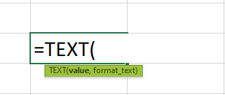
where,

value: It is the numeric value or cell reference to the numeric value we require to convert into a text string.
format_text: It is the text string that specifies the format we need to apply to the numeric value.

Unlike other functions, both the arguments mentioned in the TEXT formula in Excel are mandatory.

And here are the codes we will typically use in the second argument, format_text, to define the required formatting.

Code	Description
0	The digit placeholder, showing the irrelevant zeros.
#	The digit placeholder that hides the extra zeros.
?	The digit placeholder that provides a space for irrelevant zeros, but hides them. It usually aligns numeric values in a column at a decimal point.
.	Decimal point
,	Thousands seperator

Further, the following codes are used when we use the TEXT function in Excel with dates and times.

Code	Description
h	Hour
m	Minute when mentioned in the time format.
s	Second
d	Day
m	Month when mentioned in the date format.
y	Year
AM/PM	Time

In addition, below are a few symbols we can use in the format code, which will display at the same position in the output text where we place them in the format code.

Symbol	Description
%	Percentage
$	Dollar
&	Ampersand
/	Forward Slash
+, –	Plus and minus signs
()	Parentheses
‘	Apostrophe
:	Colon
!	Exclamation Mark
	Space Character
=	Equal Sign
^	Caret
~	Tilde

Excel VBA – All in One Courses Bundle (35+ Hours of Video Tutorials)

If you want to learn Excel and VBA professionally, then Excel VBA All in One Courses Bundle (35+ hours) is the perfect solution. Whether you’re a beginner or an experienced user, this bundle covers it all – from Basic Excel to Advanced Excel, Macros, Power Query, and VBA.

Start Learning Now

How To Use TEXT Excel Function? (With Steps)

The steps required to use the TEXT function in Excel are:

First, enter the numeric values we want to convert into text strings in a spreadsheet.
Then, type the TEXT() with the first argument as the numeric value or cell reference to the numeric value and the second argument in the required format.
Press Enter to view the numeric value as text data.

Let us understand the steps to apply the TEXT function in Excel with example.

The below table shows a number in column A along with a list of different formats in column B. Now, we need to convert the number based on the requirement.

The steps used to format text in excel are:

Step 1: To begin with, select cell C2 to display the result.

Next, enter the TEXT() as in the Formula Bar in the below image, and then, press Enter.

We will get the result as shown in the image below.

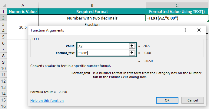
The arguments in the TEXT function in Excel are cell references to the cell containing the numeric value 20.5 and the format code for the format, Number with two decimals. Since the second argument is a text string, it is in double-quotes.

Alternatively, we can choose cell C2 and then go to Formulas > Text > Text.

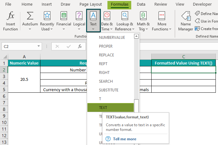
Next, the Formula Arguments window opens.

Now, fill the Value and Format_text fields and click OK to get the TEXT() formula in cell C2.

Step 2: Then, choose cell C3 and enter the TEXT() as in the Formula Bar in the below image.

Press Enter key.

Clearly, the first argument remains the same as in the TEXT() used in cell C2. But the format code will change as we need to display the numeric value 20.5 as a fraction.

Step 3: Choose cell C4 and enter the TEXT() as in the Formula Bar in the below image.

Press Enter key.

Here the first argument in the TEXT() is Excel cell reference A2, and the second argument is the format code to display the value as a percentage.

Step 4: Choose cell C5, enter the TEXT() as in the Formula Bar in the below image, and press Enter.

The text string containing the $ symbol is supplied as the second argument to the TEXT(), making the number 20.5 display as a currency.

Examples

Here are a few illustrations to show how we can effectively utilize the TEXT function in Excel.

Example 1- Prefix The Text Strings To The Newly Formatted Date Values

Consider the following table. It shows a list of laptop bags, quantities, and delivery dates in columns A, B, and C, respectively. We need to enter the delivery status as a comment in column D. Let us learn how to use text function in Excel with this example.

But first, let us see what the output will be without using the TEXT().

We would choose cell D2 and type the formula,

=B2&” units of “&A2&” were delivered on “&C2&”.”

Press Enter key.

The above result does not show the date in the required format. Instead, the date gets displayed as a number.

Now let us use the required format for the TEXT formula in Excel to ensure the date exhibited is correct. Here are the steps:

Step 1: Choose cell D2 and enter the TEXT() with the required prefix as:

=B2&” units of “&A2&” were delivered on “&TEXT(C2,”dd mmm, yyyy”)&”.”

And then, press Enter.

Step 2: Drag the AutoFill handle downwards to copy the formula into cells D3:D6.

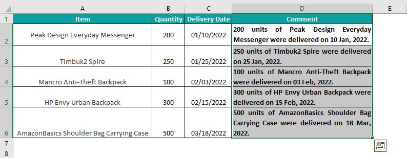
While the ampersand concatenates values and text strings, the text within the double quotes appears in the output.

Using them, we can prefix the required text string to the date, formatted using the TEXT function in Excel.

Here, the format code provided as the second argument to the TEXT() is “dd mmm, yyyy.” The term dd shows the day in two digits. And if the day is a single digit, the output will have a leading zero to display the day in two digits (refer to cell D4 in the above image).

Likewise, the code mmm indicates the month using the first three letters of the specific month.

And the term yyyy shows the year in four digits. But, on the other hand, the spaces and comma symbol appear in the output, as mentioned between the codes.

It is just one date format for the TEXT function in Excel. We can use different date formats according to our requirements.

Example 2- Join The Newly Formatted Time And Date Values

The table below shows the time and date values in columns A and B. Now, we need to combine both the values in column C.

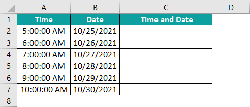
Please Note: The time and date formats in the source data are h:mm:ss AM/PM and m/d/yyyy, respectively.

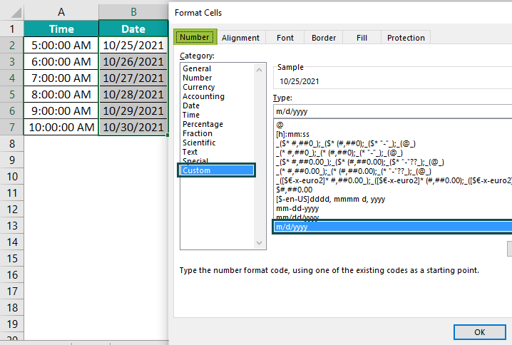
We can select cell A2:A7 and use the shortcut keys Ctrl + 1 to open the Format Cells window.

Then, in the Number tab, click the Custom option, choose the Type for the time as h:mm:ss AM/PM, and click OK.

Likewise, choose cells B2:B7 and set the Type field in the Custom category as m/d/yyyy for the dates.

Now, if we join the time and date values, say in cell C2, the output will be:

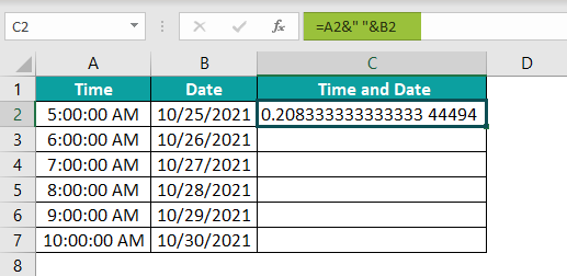
The time and date values are not in a readable format. While the time displays as a decimal value, the date is a number. However, the TEXT formula in Excel can help us achieve the required results.

Step 1: Choose cell C2. Enter the formula to format the time and date to get readable text and join them.

=TEXT(A2,”h:mm AM/PM”)&”, “&TEXT(B2,”d-mmm-yy”)

And then press Enter.

Step 2: Drag the fill handle downwards to copy the formula into cells C3:C7.

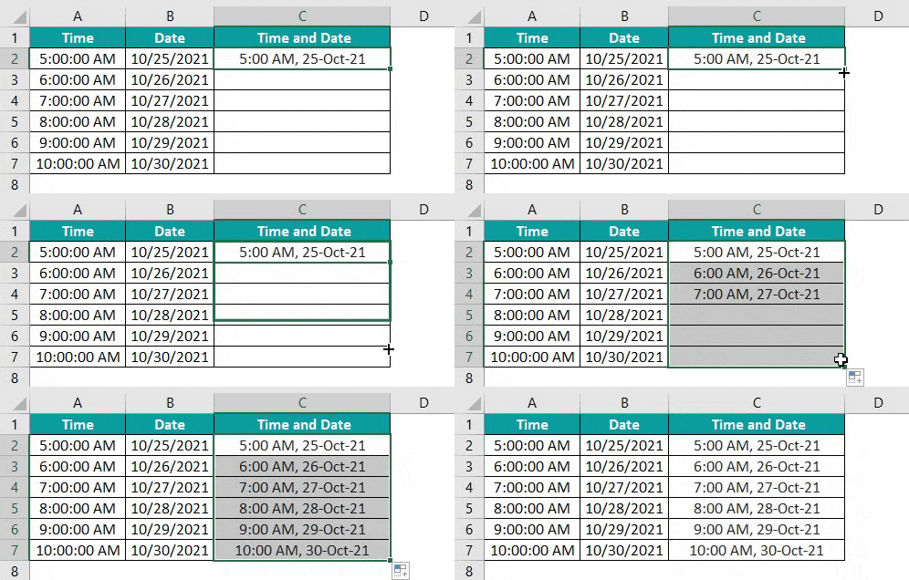
The formula uses the TEXT() twice to apply new formats to the time and date values.

The format codes are different from the ones used in the source data.

The h and mm, in the first TEXT() format code denotes the hour and minutes, with minutes in two digits. AM/PM gets displayed in the output.

And the d, mmm, and yy in the second TEXT() format code show the day, month using the starting three letters of the month and year using the last two digits of the year.

And here again, the ampersand joins the two values in each cell.

Example 3- Extract A Mobile Number From Its Scientific Notation

Suppose we enter 12-digit mobile numbers (2-digit extension and 10-digit mobile number) in our spreadsheet. Then the mobile numbers will automatically appear in the scientific notation form within the cells, though the Formula Bar will show the mobile numbers in the original format.

The reason is that Excel can show a number as it is in the cell for a maximum of 11 digits. But if the number contains 12 or more digits, Excel displays it in the scientific notation form.

Let us see how we can resolve this issue using TEXT function in Excel.

Assume the following table contains mobile numbers.

The steps to get the mobile numbers from their scientific notations using TEXT function in Excel are as follows:

Step 1: Add a new column with a header Mobile Number Displayed Using TEXT().

Choose cell B2 and enter the formula, =TEXT(A2,”############”)

Press Enter key.

Step 2: Drag the fill handle downwards to copy the formula in cells B3:B5.

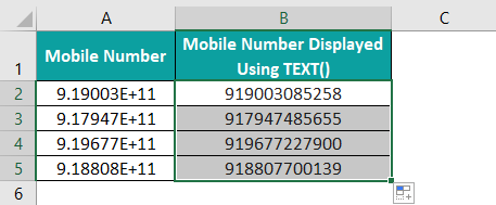
The TEXT() format code contains twelve hashes to display the 12 digits of a mobile number.

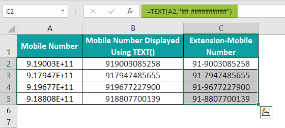
And if we require to show the 2-digit extension and the 10-digit mobile number separately, the TEXT() formula in cell C2 is,

=TEXT(A2,”##-##########”)

Once we press Enter key and drag the fill handle to copy the formula in cells C3:C5, the output will be:

Example 4- Prefix A Text String To The Initially Formatted Monetary Value

Consider the below table with income, expenses, and savings data in columns A, B, and C, respectively.

The three monetary values already have a specific format by setting the Number Format in the Home tab as Currency.

If we need to enter a comment including the total savings from cell C2, then we will enter the formula as shown in the Formula Bar depicted in the below image:

The above formula does not show the initial format of the total savings.

But, the TEXT function in Excel allows us to prefix the required text string to a monetary value while retaining its initial format.

Step 1: Choose cell C2 and use the shortcut keys, Ctrl + 1, to open the Format Cells window. Then, go to the Custom window to check the applied format since we will require it while supplying the second argument to the TEXT().

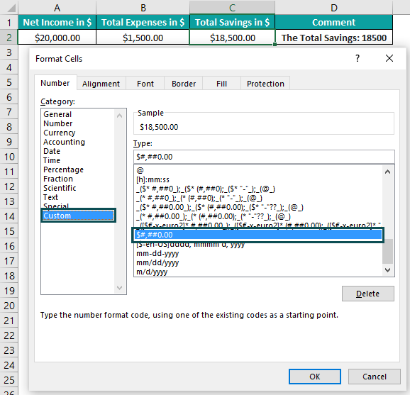
In this case, it is $#,##0.00.

Step 2: Select cell D2 and enter the below formula to prefix a text string to the initially formatted total savings value.

The formula is =”The Total Savings: “&TEXT(C2,”$#,##0.00”)

Example 5- Add Leading Zeros To Numbers

Typically, Excel removes leading zeros that are entered before a numeric value in a cell.

But sometimes, we might want to show the leading zeros, and the TEXT function in Excel enables us to achieve the required outcome.

For example, the below table shows a few numbers.

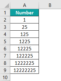
We can pad each number with leading zeros to create text strings (with 8-characters).

Step 1: Name column B as Text String – Number With Leading Zeros.

Then choose cell B2 and enter the below TEXT() as:

=TEXT(A2,”00000000″)

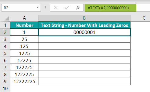
Step 2: Drag the fill handle downwards to copy the formula in cells B3:B9.

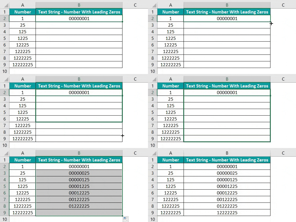
Depending on the number of digits in each number, the leading zeros get padded to it to become an 8-character string.

However, the last number appears since it already has 8-characters.

Example 6- Converting Decimal To Percentage With TEXT Function

We can use the TEXT function in Excel to convert a decimal value into a percentage. The format_text, in this case, will be ‘0.00%’ or ‘0.0%’.

For example, we need to convert the following decimal numbers into percentages.

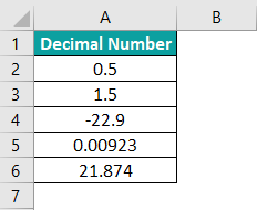
The following steps help us understand how to use text function in Excel.

Step 1: Name column B as Number In Percentage.

Then, choose cell B2 and enter the TEXT() as:

=TEXT(A2,”0.00 %”)

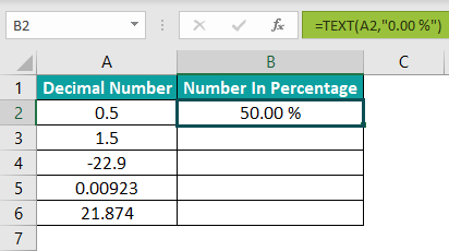
Step 2: Drag the fill handle downwards to copy the formula in cells B3:B6.

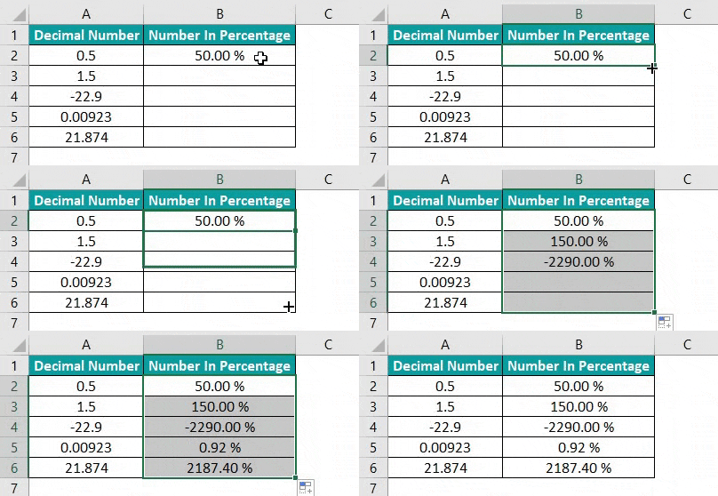
Each decimal value is multiplied by 100, with the % value added at the end.

Example 7- Converting Decimal to Fraction with TEXT Function

We can use the TEXT function in Excel to convert a decimal number into a fractional value. The format_text we need to supply as the function argument is “# ???/???”.

For example, we need to convert the following decimal numbers into fractions.

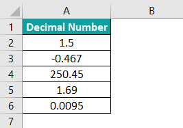
Step 1: First, choose cell B2 and enter the TEXT() as:

=TEXT(A2,”# ???/???”)

Step 2: Next, drag the fill handle downwards to copy the formula in cells B3:B6.

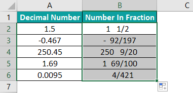
If the decimal number has a non-zero digit before the decimal point, the TEXT() with the above format code will return a mixed fraction. Otherwise, the result will be a proper fraction.

Things to Remember

Both the arguments in the TEXT function in the Excel formula are mandatory.
The second argument in the TEXT(), format_text, should be in double-quotes. Otherwise, the function returns the #NAME? error.
Ensure the date and time format codes are region-specific.
Though the TEXT() result might appear as a number, it will be a text string.
The TEXT() takes only one value and one format code as inputs.
Unlike other functions, the TEXT function is an inbuilt function available in all versions of Excel.

Frequently Asked Questions

Where is the TEXT function in Excel?

The TEXT function in Excel is in the TEXT function category under the Formulas tab.

FAQ 1

Why TEXT function in Excel is not working?

TEXT function might not be working due to the following reasons:

The format_text argument value is not in double-quotes.

For example, suppose we enter the required TEXT() formula in the target cell as:

=TEXT(B2,# ???/???)

Then, the function will throw an error.

Instead, the correct way of entering the second argument in the TEXT() is:

=TEXT(B2,”# ???/???”)

We do not use the required region-specific dates and time format in the TEXT().

For example, the format code m/d/yyyy will work for Americans. But if the users in France work on Excel with French as the preferred language, then using the format code m/d/yyyy in the TEXT() will throw an error.

It is because, in French, the day, month, and year equivalents are jour, mois, and an.

And thus, the correct format code we need to use in France is m/j/aaaa to make the TEXT() work.

What is the use of TEXT function in Excel?

The TEXT function in Excel is that we can change a numeric value into text and format it to modify how it appears in a spreadsheet. And using TEXT(), we can join numbers with text and symbols, thus making them more readable.

Download Template

This article must be helpful to understand the TEXT Function In Excel, with its formula and examples. You can download the template here to use it instantly.

Text Function in Excel Download

TEXT Function In Excel