What Is The Date Format In Excel?
The Date Format in Excel is a feature to display or enter dates in a dataset. We can format the dates in multiple ways – short or long, as per the requirement. The default Date Format in Excel is present in the “Control Panel” of the system. It is found in the “Number” group of the “Home” tab.
For example, in cell A1 the date is 01-01-2022, and we want to change the date to the Long Date.

Select cell A1 > go to the “Home” tab > go to the “Number” group > click on the “Number Format” drop-down > select the “Long Date” option.
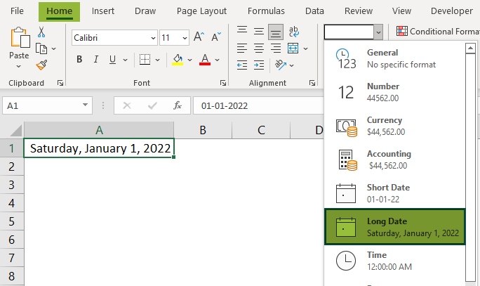
The output is shown above. The short date is converted to a long date.
📥Download the ready-to-use Excel template to practice this tutorial yourself.
Date Format in ExcelKey Takeaways
- The Date Format in Excel helps to change the dates in desired formats, short or long.
- The DATEVALUE formula converts the data into a number format.
- We can identify the default date in Excel as it will have an “*” symbol at the start of the default date format.
- “CTRL+1” is the shortcut key combination to open the “Format cells” window to customize the Date Format in Excel.
- We cannot convert the dates before January 1, 1900, to text in excel because it will not read negative numbers and remain in the same format.
Code Of Date Format In Excel
We display the Code Of Date Format in Excel i as a day (d), month (m), and year (y). We will understand these three codes in detail.
- The Day Format(d) –
| Code | Explanation | Result |
|---|---|---|
| d | Day with Single Digit | 1 |
| dd | Day with Double Digit | 01 |
| ddd | Day Short Name | Mon |
| dddd | Day Full Name | Monday |
- The Month Format(m) –
| Code | Explanation | Result |
|---|---|---|
| m | Month with Single Digit | 1 |
| mm | Month with Double Digit | 01 |
| mmm | Month Short Name | Jan |
| mmmm | Month Full Name | January |
- The Year Format(y) –
| Code | Explanation | Result |
|---|---|---|
| yy | Year with Double Digit | 22 |
| yyyy | Year with Full Digit | 2022 |
How To Change Date Format In Excel?
We can change the Date Format In Excel in multiple ways, namely,
- Apply Default Format of Long Date
- Short Date Format
- Change The Date Excel Format Using “Custom” Option.
- Apply Different Types of Customized Dates Format in Excel.
- Convert Text Values Representing Dates to Actual Dates.
- Change The Date Format Using The “Find and Replace” Box.
- The DATEVALUE formula converts the date into a number format.
#1 – Apply Default Format Of Long Date In Excel
We will Apply Default Format Of Long Date using the Long Date format technique.
In the table below, the data is,
- Column A contains the Date.
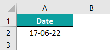
The steps to apply the Long Date format Excel technique are as follows:
1: Let us select cell A2.
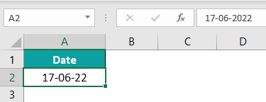
2: Then, go to the “Home” tab > go to the “Number” group > click on the “Number Format” drop-down > select the “Long Date” option.
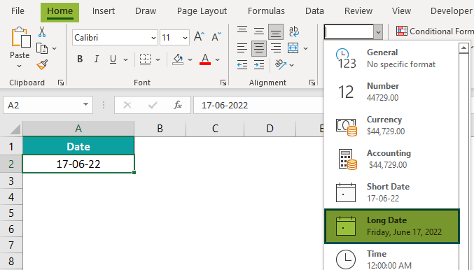
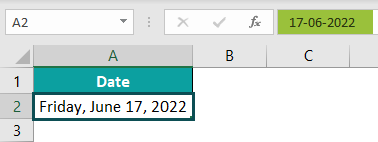
The output is shown below. The date is “Friday, June 17, 2022”.
#2 – Short Date Format In Excel
We will change the format using the Short Date Format Excel technique.
In the table below, the data is,
- Column A contains the Date.

The steps to apply the Short Date Format Excel technique are as follows:
1: We will select cell A2.

2: Now, go to the “Home” tab > go to the “Number” group > click on the “Number Format” drop-down > select the “Short Date” option.
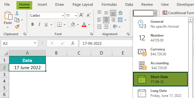
The output is shown below. The date is “17-06-2022”.

#3 – Change The Date Excel Format Using “Custom” Option
We will Change The Date Excel Format Using “Custom” Option.
In the table below, the data is,
- Column A contains the Date.
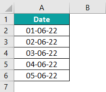
The steps to apply the Short Date Format Excel technique are as follows:
1: Let us select cell range A2:A6.
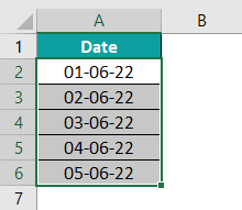
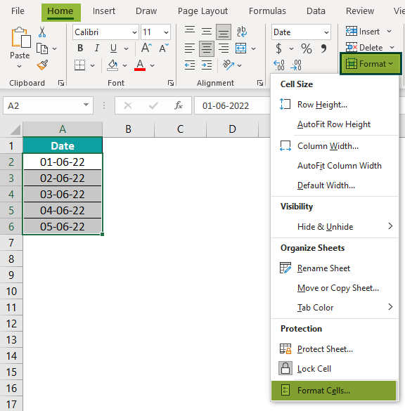
2: Now, go to the “Home” tab > go to the “Cells” group > click on the “Format” drop-down > select the “Format Cells…” option, as shown below.
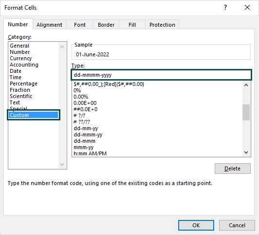
3: In the “Format Cells” window, select the “Number” bar > go to the “Category:” group on the left side > select the “Custom” option > go to the “Type:” group on the right side > click on the “dd-mmmm-yyyy” option or manually type in the “Type:” field, as shown below.
4: Then, click on “OK”. The output is shown below.

#4 – Apply Different Types Of Customized Dates Format In Excel
We will Apply Different Types Of Customized Dates Format In Excel as follows:
- Format 1: dd-mm-yy
- Format 2: dd-mm-yyy
- Format 3: ddd-mmm-yyyy
- Format 4: dddd-mmmm-yyyy
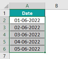
We will apply all the above formats to the following table.
- Column A contains the Date.

- Format 1: dd-mm-yy
The steps to apply the Date Format using the “Custom” option technique are as follows:
1: First, select the cell range A2:A6.

2: Next, select the “Home” tab > go to the “Cells” group > click on the “Format” drop-down > select the “Format Cells…” option, as shown below.

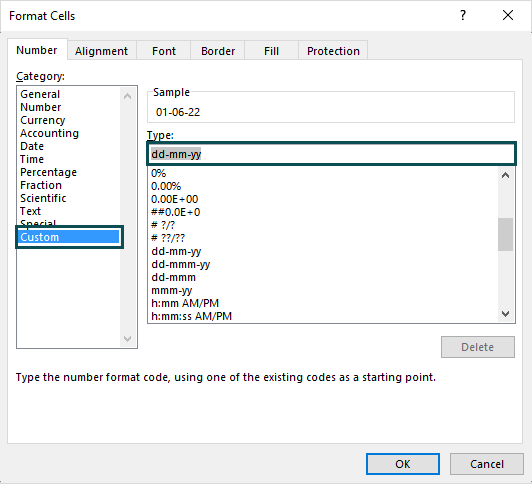
3: In the “Format Cells” window, select the “Number” bar > go to the “Category:” group on the left side > select the “Custom” option à go to the “Type:” group on the right side > click on the “dd-mm-yy” option or manually type in the “Type:” field, as shown below.
4: Finally, click on “OK”. The output is shown below.

- Format 2: dd-mm-yyy
The steps to apply the Date Format In Excel using the “Custom” option technique are as follows:
1: Let us select the cell range A2:A6.

2: Next, go to the “Home” tab > go to the “Cells” group > click on the “Format” drop-down > select the “Format Cells…” option, as shown below.

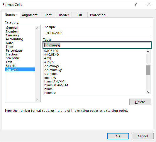
3: Select the “Number” bar, in the “Format Cells” window > go to the “Category:” group on the left side à select the “Custom” option à go to the “Type:” group on the right side > click on the “dd-mm-yyy” option or manually type in the “Type:” field, as shown below.
4: Then, click on “OK”. The output is shown below.
- Format 3: ddd-mmm-yyyy
The steps to apply the Date Format using the “Custom” option technique are as follows:
1: We will select the cell range A2:A6.

2: Go to the “Home” tab > go to the “Cells” group > click on the “Format” drop-down > select the “Format Cells…” option, as shown below.

3: When the “Format Cells” window opens à select the “Number” bar à go to the “Category:” group on the left side à select the “Custom” option à go to the “Type:” group on the right side à click on the “ddd-mmm-yyy” option or manually type in the “Type:” field, as shown below.
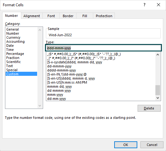
4: Press the “OK” button, we will get the following output.

- Format 4: dddd-mmmm-yyyy
The steps to apply the Date Format using the “Custom” option technique are as follows:
1: Select the cell range A2:A6.

2: Next, go to the “Home” tab > go to the “Cells” group > click on the “Format” drop-down > select the “Format Cells…” option, as shown below.

3: In the “Format Cells” window, select the “Number” bar > go to the “Category:” group on the left side > select the “Custom” option > go to the “Type:” group on the right side > click on the “dddd-mmmm-yyyy” option or manually type in the “Type:” field, as shown below.
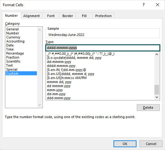
4: Press the “OK” button. The output is shown below.

[Note: When we add the date formats manually in the “Custom” option, it gets saved in Excel. So, the next time we open Excel, we can select the formats instead of adding them again].
#5 – Convert Text Values Representing Dates To Actual Dates
We will Convert Text Values Representing Dates To Actual Dates.
In the table below, the data is,
- Column A contains Date in Text Date Format.

The steps to apply the Actual Date Format are as follows:
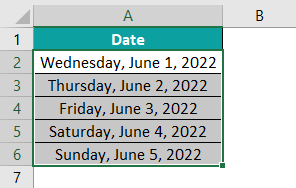
1: Let us select cell range A2:A6.

2: Go to the “Home” tab > go to the “Number” group > click on the “Number Format” drop-down > select the “Long Date” option.

The output is shown below. The dates get formatted to the Long Date Format Excel.
#6 – Change The Date Format Using The “Find and Replace” Box
We will Change the Format Using The “Find and Replace” Box, where the technique replaces “-” with “/” in the Date Format In Excel.
In the table below, the data is,
- Column A contains the Date.

The steps to apply the Find and Replace technique on the Actual Date Format are as follows:
1: We will select cells A2:A6.

2: Then, select the “Home” tab > go to the “Editing” group > click the “Find & Select” drop-down > select the “Find” option, as shown below.

3: When the “Find and Replace” window pops up > enter the “-” symbol in the “Find what:” field and the “/” sign in the “Replace with:” field > click on the “Replace All” button.

The output is shown below.

Excel Date Format Not Working
The Date Format in Excel may not work for the following reasons,
- The cell size is not wide enough for the entire entered date –
If we enter the date longer than the cell’s size, the date will appear as “#####”. The solution is to resize or manually increase the column width, as required.
- The negative number is entered in Date format –
If we enter the date, which is the negative value, the date will appear as “#####”. The solution is to switch the 1904 date system from the “Excel Options” in the “File” tab or use the Excel TEXT function to display negative dates.

Frequently Asked Questions (FAQs)
The default format is the set Date Format in Excel. We can view it as follows: select the “Home” tab > go to the “Cells” group > click on the “Format” drop-down > select the “Format Cells” option. The “Format Cells” window pops up, click the “Numbers” bar > go to the “Category” group on the left, and click on the “Date” option. In the “Type:” group, we will see the default date format with the “*” Asterisk sign, as shown in the following image.
The set default Date is,
14-03-2012
March 14 2012
We can convert Date Format into Excel in two methods as follows:
Method 1: Format Cells Dialog.
The step-by-step process to convert Date Format using the Format Cells Dialog box are:
1. Select the cell to be formatted, here, cell A2.
2. Select the “Home” tab à go to the “Cells” group à click on the “Format” drop-down à select the “Format Cells…” option. [Alternatively, press the shortcut keys “CTRL+1” to open the “Format Cells” window].
3. The “Format Cells” window pops up. Select the format in which we want to Convert the Date in Excel. In this case, we have selected the “General” format from the “Number” menu bar “Category” list.
The output is shown below.
Method 2: Excel DATEVALUE function
We can use the DATEVALUE() function to convert the Date Format in Excel.
The step-by-step process to convert Date Format in Excel using the DATEVALUE function are:
1. Select cell A2 to apply the DATEVALUE function.
2. Enter the DATEVALUE formula =DATEVALUE(“17-06-2022”) in cell A2.
3. Press the “Enter” key. The output is ‘44729’, as shown below.
The step-by-step process to change the Date Format in Excel are,
1. Select the cell which has the date.
2. Select the “Home” tab > go to the “Cells” group > click on the “Format” drop-down > select the “Format Cells…” option
3. The “Format Cells” window pops up.
4. Select the “Number” bar > select the “Date” option from the “Category:” group > select the desired date format from the “Type:” group > click on “OK”.
Download Template
📥Download the ready-to-use Excel template to practice this tutorial yourself.
Date Format in ExcelRecommended Articles
This has been a guide to Date Format In Excel. Here we change date formats, short date, long date, & custom dates with examples & downloadable excel template. You can learn more from the following articles –

Leave a Reply