
What Is Name Range In Excel?
While working in Excel, it is common to refer to cells by their names, such as A1, B4, D3, etc. However, users can give custom names to a cell range instead of referring to cells with their default names. Therefore, defining the names for cells or a cell range is called Named Range in Excel. We can easily work with Excel by defining the name for cells or a cell range since we can move across cells using the names instead of navigating through them.
For instance, consider the below table with sales and cost data in column A and the values in column B. The table also has profit value which is obtained by subtracting Sales-Cost. We need to use the following steps to understand Name Range in Excel.
Use this Name Range In Excel Template to follow along with the examples in this article.
Download Excel Template
In the formula bar, we can see the formula as =B2-B3. After we name cell B2 as ‘Sales’ and B3 as ‘Cost,’ we can see the named cell references in the profit calculation cell.

Naming cells also help users understand the actual function. For instance, when we click on cell B4, users can instantly understand that the cell shows the value of profit obtained by using the formula, ‘Profit = Sales-Cost’ when compared with the original references, ‘=B2-B3.’
Key Takeaways
- Named Ranges in Excel can be created by using the Excel name box.
- This feature makes our work easier; we need not navigate the separate worksheet to select the targeted range if the named range is already created for the required range of cells.
- Dynamic named ranges make the drop-down list, and any addition in the specified range will be updated dynamically.
- The top row headers are selected as names for the following cell.
How To Create A Name Range In Excel?
We can create a name range in Excel by using four different ways. However, before we look at the methods, we must know the rules we must follow before creating a name range in Excel. They are:
- The name should not start with a number. It should always start with the text, underscore (_), or backslash (/).
- It should not have a space or special characters except underscore (_).
- It needs to be unique.
- We cannot name range in Excel only with the cell reference. For instance, AZ1 is a cell reference, so we cannot use it.
- We cannot use single letters such as ‘R’ or ‘C’ because these are the characters used to select rows or columns for the currently selected cell when we enter them in the name box.
- We can name each cell using a maximum of 255 characters.
- The name cannot be case-sensitive.
For instance, the function treats ‘January,’ ‘january’, and ‘JANUARY’ as same.
Please Note: We can view the actual (original) cell references by pressing the F2 key. This key activates the edit mode. Let us understand the tool in detail in the following sections. Now, let us look at the 4 different ways to name a range in Excel.
Create Name Range Using Name Box
We can name a cell or range using an Excel name box. When we select any of the cells at the top left corner, we can see the name box displaying the Excel cell reference, as shown in the image below:

Users can name a cell or a range according to their requirements. In our example, let us name the cell ‘Product_Cell.’

Similarly, we can also name a range in Excel using the name box. In our example, let us select the entire table, A1:D4, and name it ‘Product_Sales.’

Create Name Range Using Define Name
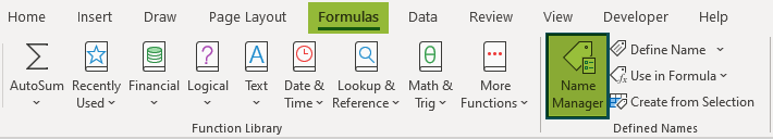
Under the Formulas tab, click on the Define Name option from the Defined Names group.

When we click the option, the New Name window pops up.

Let us understand each of the four options in the window to understand better.
Name: We should type the required name in this box. So, let us type the name ‘Product_Table’ in this section.

Scope: By default, the scope will be at the workbook level. We can choose from the drop-down options to change it to a different worksheet.
Comment: This is the comments section where users can add the reason for naming a cell or a range. These comments help future users understand the worksheet and allotted names.

Refers To: Here, we need to choose the cell range that is being named.
Since we are naming the entire table in our example, choose the cell range A1:D4 in this section.

Select OK to name range in Excel.
Please Note: As soon as we choose the cell range, it becomes an absolute reference by default.
Now, we can use the name ‘Product_Table’ anywhere in the workbook.
For instance, if we type =product in any of the cells, excel will list out the name in the options as shown in the image below:

When we select the name prompted by excel, it will highlight the cell range.
In our case, excel highlights the range, A1:D4.

To insert the table into the worksheet, press Enter key.
Excel returns the table as shown in the image below:

Apart from displaying the range’s name, we can also see that the table has a blue line. It indicates that the table has been imported.
Create Name Range Using Name Manager
Select the Name Manager option from the Formulas tab.
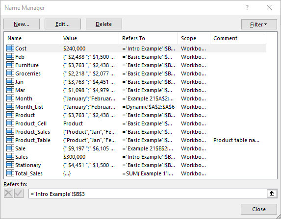
The Name Manager window opens with the list of names we have created.

Click on the New tab to open the New Name window.
As discussed earlier, we can fill the options in the window and create names for a cell range.
Create Name Range Using Create from Selection
So far, we have learned how to name a cell or a range in Excel using the name range in Excel feature. But, using this method, we can name multiple ranges with just a click.
Let us learn the method using the following example. The below table lists the products and the amount spent in the first quarter in columns A and B, respectively.

Let us learn how to name ranges in Excel.
- For instance, the range, B2:D2, is about the product, ‘Furniture’ and the amount spent.
- So, let us name this range as Furniture.
- Similarly, we can name cell ranges B3:D3 and B4:D4 for stationery and groceries data.
- Likewise, we can name tables using the column header. For example, we can name the cell range from B2:B4, C2:C4, and D2:D4 as Jan, Feb, and Mar, respectively.
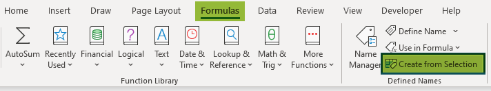
- Now, select the data range from A1:D4 and click on Create from Selection option under the Formulas tab.
The Create from Selection window pops up.

We have data headers in the top row and the left column. So, by default, it has selected both options.
Next, click OK to create the name ranges.
Now, go to the Formulas tab and click on the Name Manager option.
The Name Manager window pops up with the list of named ranges in Excel.

We have 6 different named ranges. So whenever we want to sum values of Jan month, we have to open the SUM Excel function and enter the name ‘Jan’.

As we can see in the above image, ‘Jan’ month refers to the cell range B2:B4.
In this way, we can create multiple named ranges in different ways.
So, we have learned how to create a name range in Excel.
How To Use Name Range In Excel?
Let us understand the feature better with the following examples.
Example #1 – Find Percentage Of Grand Total
For instance, we have the following monthly sales data in an Excel spreadsheet.

We need to find the percentage share of each month for calculating the total sales. Generally, we first calculate the sum of all the months, and from that month, we calculate the percentage share of each month. We use the same method, and it is highlighted in the following image.

Step 1: SUM($B$2:$B13$) is the total sales formula for all the months.
The formula may be confusing, but with the help of name range, we can easily create the total sales name range.
Step 2: Under the Formulas tab, click on the Define Name option.
The New Name window pops up.
Let us type the name Total_Sales in the Name: box.

Step 3: Similarly, enter the following formula in the Refers to: box as shown in the image:
=SUM(‘Example 1’!$B$2:$B$13)
The sum of all the values from B2:B13 will be calculated instantly.

Step 4: Click OK to name the range as ‘Total_Sales’.

Step 5: In the percentage share calculation formula, apply this named range as shown in the following image.

Instead of the SUM function, we have used named range, and the result is the same as the previous one.
Example #2 – Apply Names To Existing Formula
We can still name ranges even if we have already applied the formula with regular references.
Step 1: For instance, we have applied the SUMIF function in the following image to get the particular month’s sales.

We have used two ranges here, i.e., A2:A13 for months and B2:B13 for sales.
Step 2: Now, let us give a name for the range A2:A13 as ‘Month’.

Step 3: Similarly, give a name for the range B2:B13 as Sale.

Step 4: Now, we need to apply the names to the existing formula in cell E2.
So, select cell E2, go to the Formulas tab and click on Define Name.
We can see two options in the drop-down list. Click on Apply Names…

The Apply Names window pops up. We can see all the names we have created in the workbook.

Step 5: From the list, the named range in Excel feature can be applied to ‘Month’ and ‘Sale.’ So, select these two and click on OK.

Step 6: When we click OK, it will update the formula with named ranges.

This way, we can use named ranges in Excel to work efficiently.
Delete Name Range In Excel
We know that creating a name range in excel is simple. Similarly, we can delete name range in Excel using Name Manager. Let us learn the steps involved.
Step 1: Go to the Formulas tab and click on Name Manager.
Step 2: This will show us the list of names.
Step 3: Select the named range that we want to delete and hit the button Delete on top. If we want to delete multiple named ranges, hold the control key and select the named ranges by clicking on them.
Step 4: Once the selection is made, we can hit the Delete button, and all the selected named ranges will be deleted.
Step 5: However, if we have too many named ranges to deal with, we can use Filters at the top.

Filters offer a variety of options like choosing named ranges within the worksheet scope, workbook scope, names that have errors, etc.,
As mentioned, we can delete name range in Excel.
Dynamic Name Range In Excel
When we create a named range, it is static and will not be updated when the new list is added to the range. For instance, in the following image, we created a drop-down list using a named range.

Step 1: We have named the cells A2:A6 as Month_List and used the same name while creating a drop-down list.

Step 2: However, when we added the month name Jun in cell A7, we could see that the drop-down list is not updated.

It is because the named range ‘Month_List’ is not dynamic and any new entries added to the list will not be updated.
We need to make the named range dynamic.
Step 3: So, go to the Formulas tab and click on Name Manager from the Defined Named group.
Step 4: It will bring the list of all the named ranges. For example, select the named range Month_List and click on the Edit option.

Step 5: Now, enter the following OFFSET Excel formula in the Refers to box.
=OFFSET(A2,0,0,COUNTA(A2:A13),1).

Click on OK.
Step 6: Now, enter any values from cells A2 to A13, and the drop-down list will be updated dynamically.

We have added 4 more months from cells A7 to A10, and the drop-down list dynamically shows the newly added months.
Break Down of the Formula:
The formula denotes the following:
- =OFFSET(A2,0,0,COUNTA(A2:A13),1)
- =OFFSET(A2: The OFFSET function starts the offset from cell A1.
- =OFFSET(A2,0,0: It moves down 0 rows and 0 columns.
- =OFFSET(A2,0,0,COUNTA(A2:A13): COUNTA Excel function will return the number of rows we have data in cell A2:A13, and then the OFFSET function offsets the same number of rows starting from cell A2.
- =OFFSET(A2,0,0,COUNTA(A2:A13),1): Since we are offsetting only one column, the last argument will be 1.
Like this, we can create a dynamic drop-down list by making the named range dynamic.
Important Things To Note
- Names should not contain any special characters and spaces.
- Names should start with an alphabet only.
- Only underscore (_) and backslash (/) can be used as special characters in a name.
- The name is not case-sensitive, so the names ‘Apple’, ‘apple’, and ‘APPLE’ are treated as the same.
- The shortcut key to bring the list of names is F3.
- We can press the shortcut keys Ctrl + F3 to create a new name range.
- The shortcut keys in Excel to create a name range from the current selection are Ctrl + Shift + F3.
Frequently Asked Questions (FAQs)
We can name range in excel with ease.
For instance, consider the table with the list of fruits in column A.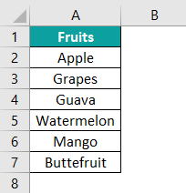
To name the entire table, i.e., A2:A7, we need to follow the below steps;
● Select the entire table
● Type the desired name in the name box
In our example, let us type the range as ‘Fruit_List.’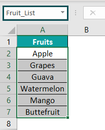
Another advantage of the feature is that we can search for the cell range A2:A7 Fruit_List.
Similarly, we can create name range in excel for a specific cell reference or a range.
Using named ranges in Excel, we can easily refer to cells from different worksheets. It speeds up the work and makes it more efficient.
Apart from this, with the help of structured named ranges, calculations can be easily understood when a new user takes over the file.
We can edit name range in excel with the following steps:
Step 1: Go to the Formulas tab and click on Name Manager option.
The Name Manager window with a list of created name range in excel pops up.
We should click on the Edit option to make the required changes.
Likewise, we can edit name range in excel.
We can name range in excel using selection. For instance, consider the following table with revenue earned in Jan, Feb, Mar, and Apr in columns A, B, C, D, and E, respectively.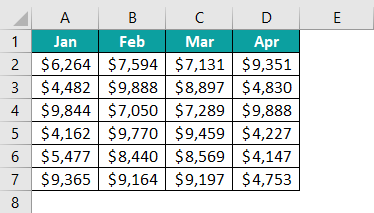
If we want to create a name range for each column by using the column headers, then we have to select the data range.
So, go to the Formulas tab and click on Create from Selection.
The Create Names from Selection window appears. Choose the Top Row option.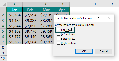
Click OK to create a name range using selection.
Use this Name Range In Excel Template to follow along with the examples in this article.
Download Excel TemplateRecommended Articles
Continue with these related resources when you want the next practical step in this topic.
- Cell References in Excel
- Relative References in Excel
- Mixed References In Excel
- 3D Reference in Excel
- Structured References In Excel
Explore the full Excel Reference Functions guide or browse Excel Resources.