
What Is SUM Excel Function?
The SUM function in Excel enables users to add individual numeric values, cell references, ranges, or all three together using the formula =SUM(). Likewise, using the Auto Sum formula in Excel, i.e., “∑” automatically adds all the numeric values listed in a particular row or column. It is part of the Math and Trigonometry function.
For example, the following image shows two numbers, 10 and 20, in cells B1 and C1. We can add both numbers using the SUM formula in the merged cells B2 and C2.
=SUM(B1,C1)

The result comes as 30.
Use this SUM Excel Function Template to follow along with the examples in this article.
Download Excel TemplateKey Takeaways
- Using the SUM formula, users can add individual numeric values, cell references, ranges, or all three combined in Excel.
- It automatically updates when we include more rows and columns or delete any rows and columns.
- The Auto Sum function, i.e., “∑” automatically sums all the numeric values listed in a specific row or column.
- The function makes output as easy to understand in numerical form, eliminates the difficulties of manually adding the values, ignores the empty cells and text values, and adds all cell ranges, whether they are contiguous.
Syntax Of The SUM() Excel Formula

The image below explains the arguments accepted by the SUM function in Excel:
- number1 = The first numeric value that you want to add. This is the mandatory argument.
- number2 = The second numeric value that you want to add. This is the optional argument.
How To Use SUM Excel Function?
Let us look at a basic SUM excel function example to understand better how to use the SUM formula:
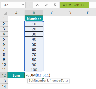
The image below depicts a series of numbers 10 to 100. We will try to sum up the numbers with the SUM function.
In the table, the data is reflected as below:
- Column B shows Numbers – 10, 20, 30, 40, 50, 60, 70, 80, 90, 100
- Cell B12 calculates the sum

The steps to use SUM() Excel Function to add the given numbers are as follows:
- First, we will choose the cell where we want the result to show up. Cell B12 would be the cell in this case.
- Next, we will enter the SUM formula in cell B12.
- Select the array which ranges from the starting cell address to the ending cell address of the table, i.e., cell references, “B2:B11”.
=SUM(B2:B11)
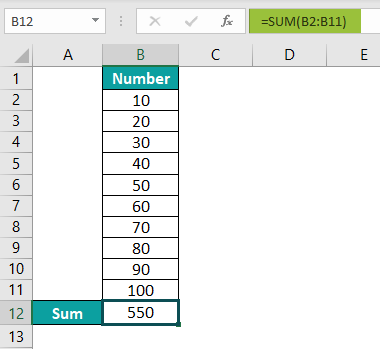
- After entering each value in the preceding step, press the “Enter” key. The results are shown in cell B12 as 550 in the image below.

Examples
Let us look at some more advanced SUM excel function examples to understand how it works:
Example #1 – SUM a Column In Excel
The image below depicts school data of class 4 students, including their names, subjects, and marks. Here, we will try to calculate the total marks of all students in each subject using the SUM function.
In the table, the data is reflected as below:
- Row 1 shows the names of the students
- Column A shows Subjects
- Column B contains marks of John
- Column C contains marks of Ron
- Column D contains marks of Harry
- Column E contains marks of Jenifer
The steps to calculate the total marks of all students in particular subjects are as follows:
Step 1: First, we will choose the column where we want the result to show up. Column F would be the column in this case.

Step 2: Enter the formula that needs to add values from all columns. Since marks of Maths of all students are present in row 2. Start adding first the marks of John from cell B2.

Step 3: Second, add the marks of Ron from cell C2.

Step 4: Third, add the marks of Harry from cell D2.

Step 5: Fourth, add marks of Jenifer from cell E2. The complete formula will be:
=SUM(B2,C2,D2,E2)

Step 6: After entering each value in the preceding step, press the “Enter” key. The results are shown in cell F2 of the image below.

Step 7: Press the “Enter” key. Then, drag the formula downwards to cell F6 to get the results for all students.

Example #2 – SUM a Row in Excel
The image below depicts the deposit and withdrawal of John’s account for five days. Next, we will calculate the total amount using the SUM function in Excel.
In the table, the data is reflected as below:
- Row 1 shows the names of the students
- Column A shows the Date of transactions
- Column B contains Item, i.e., details of transactions
- Column C contains the Amount
The steps to calculate the total amount are as follows:
Step 1: First, we will choose the cell where we want the result to show up. Cell C7 would be the cell in this case.

Step 2: Next, enter the formula that needs to add values from all rows. Since the amount is present in column C, first add the amount of John’s account from cell C2.

Step 3: Second, add the amount of John’s account from cell C3.

Step 4: Third, add the amount of John’s account from cell C4.

Step 5: Fourth, add the amount of John’s account from cell C5.

Step 6: Fifth, add the amount of John’s account from cell C6. The complete formula will be:
=SUM(C2,C3,C4,C5,C6)

Step 7: After entering each value in the preceding step, press the “Enter” key. The results are shown in cell C7 as 100 of the image below.

Example #3 – Sum Filtered Cells
At times some data needs to be filtered or hidden in a worksheet. An usual SUM formula does not work because it adds all the values in the specified range, including the filtered cells.
If we want to sum only the filtered (visible) cells, we need to organize the data by turning on the Excel Total Row feature. We then select the SUBTOTAL function to add the filtered data and ignore hidden cells.
Another way to sum up the filtered cell is to manually click the Filter button on Data Tab and enter the SUBTOTAL formula.

=SUBTOTAL(function_num,ref1,[ref2],…)
- function_num = The number determines the subtotal function from 1 to 11 or 101 to 111.
- ref1, ref2,… = It is the cell references or ranges we want to subtotal.
For example, the image below depicts the product names and quantity. Here, we will attempt to calculate the sum of the filtered cells, i.e., cosmetics, using the SUBTOTAL function.
In the table, the data is reflected as below:
- Column A shows the Products (grocery and cosmetics)
- Column B contains the Quantity
The steps to calculate the total quantity of cosmetics are as follows:
Step 1: First, we will choose the cell where we want the result to show up. Cell B11 would be the cell in this case.

Step 2: Now create a filter for products and choose cosmetics only.

Step 3: Next, enter the formula to add value from all rows. Since the quantity is present in column B, add the first argument of the SUBTOTAL function, i.e., the SUM excel function denoted by number 9 (include hidden cells manually) or 109 (exclude hidden cells) in SUBTOTAL suggestions reflected in cell B11. Both numbers omit rows that have been filtered out.

Step 4: Select the ref1, which ranges from the starting cell address to the ending cell address of the table, i.e., “B3:B10”. We will use 109 as the ref1 argument as we want to add cosmetics (visible cells) to the total. The complete formula will be:
=SUBTOTAL(109,B3:B10)
Step 5: After entering each value in the preceding step, press the “Enter” key. The results are shown in cell B11 as 480 of the image below.

Sum Excel Function Not Working
A user may encounter issues while executing the SUM formula in excel. Here are a few ways to fix such problems:
- Match the supplied cell range supplied with the dimensions of the source.
- Always format the cell containing the output as a number.
- Enter correct syntax formats
- Avoid extra spacing between the arguments of the formula.
- Add values manually by default.
Important Things To Note
- The “#VALUE!” error in the SUM function occurs when the text string is more than 255 characters long.
- The SUM function automatically ignores empty cells and the cells that contain text.
- It will return an error if the argument contains an error.
- The arguments can be constants, numeric values, ranges, or cell references.
- The output is numeric for the sum of values.
Frequently Asked Questions (FAQs)
Below is the step by step process of adding numbers using the SUM function:
1. Select a blank cell.
2. Type the formula =SUM(….
3. Select the range of the data / or select the individual values you want to add.
4. Press “ENTER.”
For example, the image below shows multiple values. Here, we will calculate the sum of these numbers using the SUM function and Auto Sum “∑.”
1. Column A shows the integer numbers and decimal numbers
2. Enter the SUM formula in cell A9.
=SUM(A2:A8)
3. Press the “Enter” key. The results are shown in cell A9 as ‘12952.304’ of the image below.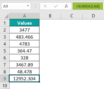
The “Auto Sum” button in the “Formula” tab also adds up the values with just one click, as shown in the following image. It adds the value above cell A9 chosen for the result.
The formula shows up automatically by the click.
=SUM(A2:A8)
The result is as same as shown in the above image.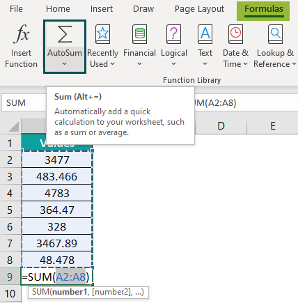
The SUM function is a means to add all numbers in a range of rows or columns and returns the output. It is a built-in Excel function listed under the Math & Trig Function.
=SUM(number1,[number2],…)
One can activate the SUM formula in Excel using the following steps:
1. Select the empty cell which will contain the result.
2. Select the “Formulas” tab.
3. Click on the “Math & Trig” option.
4. Select the “SUM” option.
5. The “Function Arguments” window pops up.
6. Enter the value in the “number 1” and “number 2” as the number of arguments.
7. Click OK.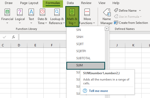
Use this SUM Excel Function Template to follow along with the examples in this article.
Download Excel Template