Index Match in Excel

What Is INDEX MATCH In Excel?

INDEX MATCH is an Excel function that combines the INDEX and MATCH formulas to allow users to retrieve the value in advanced lookups. The former fetches the value in a table depending on the column and row number, whereas the latter returns the relative position of a value in a row or column. Moreover, it can lookup values from left to right and right to left across a range of cells. As a result, it is a more suitable alternative for the VLOOKUP function.

For instance, we can use the INDEX MATCH function in Excel to find an employee’s name based on their employee ID using the data below:

First, we will create a reference cell, i.e., D2, containing Employee ID (11 in this case). Next, we will try to fetch the name of the employee in cell E2 by entering the formula:

=INDEX(B2:B9,MATCH(D2,A2:A9,0))

INDEX function looks for the employee’s name in B2:B9 based on the row number provided in the MATCH function for the employee ID 11 in cell D2. The function returns the result as ‘Mirel,’ which is the employee’s name with the ID 11 in the table array.

What Is INDEX MATCH in Excel?

The INDEX MATCH function in Excel works for horizontal and vertical data tables. Thus, it works as an alternative to the VLOOKUP function.
Unlike VLOOKUP, which works only from left to right, the INDEX MATCH function can lookup values throughout an array from right to left and left to right.
The INDEX MATCH function combines INDEX and MATCH formulas to get the desired result in . We can use the MATCH function in conjunction with the INDEX function to dynamically obtain the row and column numbers.

Syntax – INDEX + MATCH Function

The INDEX MATCH is a combo of the INDEX and MATCH formula. Therefore, we can use it to get the desired result for the lookup value.

Let us understand the syntax of these two functions one by one:

#1 – INDEX Function

Reference: It can be a single cell range or a collection of non-adjacent cell ranges.
Row_Number: The first argument from the Array, from which we need to fetch the value of the exact row number.
[Column Num]: This is an optional argument from the Array, which we use to fetch the value from the specified row and column.
[Area_Num]: Again, this is an optional argument, which we can use for multiple ranges for an argument. We can provide the area number by selecting the reference from all the available ranges.

#2 – MATCH Function

The MATCH function has three arguments. Below is the image of the same:

Lookup_Value: The value whose position you want to locate in the lookup array (second argument). It is a mandatory argument.
Lookup_Array: This will be either range or table array where you search for the lookup value. It is also a mandatory argument.
[Match_Type]: It is an optional argument and the matching criteria you need to define for the lookup value. It can be:

1 = It will look for the largest value, either less than or equal to the lookup_value you have provided, and return the approximate match. It requires lookup_array to be arranged in the ascending order (lower to higher or A to Z).

0 = It will look for and return the exact match to the lookup_value, irrespective of how the data is arranged or sorted.

-1 = This will search for the smallest value, either greater than or equal to the lookup_value you have provided, and return the approximate match. It requires the lookup_array to be arranged in descending order (higher to lower or Z to A).

Excel VBA – All in One Courses Bundle (35+ Hours of Video Tutorials)

If you want to learn Excel and VBA professionally, then Excel VBA All in One Courses Bundle (35+ hours) is the perfect solution. Whether you’re a beginner or an experienced user, this bundle covers it all – from Basic Excel to Advanced Excel, Macros, Power Query, and VBA.

Start Learning Now

How To Use Index + Match Excel Function?

INDEX function searches for the value within the array based on the row and column number provided.

For example, below is the sales data for different U.S. states in different years:

We will find the sales value for the state BG for 2018.

Below are the steps to get the result:

Step 1: Enter the INDEX function in cell K3.

Step 2: We need to select the table array for the array argument, i.e., from B2:I10.

Step 3: Enter the row number from the array to fetch the cell value. Here, we are trying to find the value for the state BG; hence row number will be 4 (5^th row in excel).

Step 4: We are also looking for the value for a particular year. So, we need to provide the column number for the table array. Here, we are trying to find the value for 2018, and the column number will be 4.

This finishes the INDEX formula. Now, close the bracket, and hit the enter key to get the result, i.e., 3,895 for BG.

We have manually provided row and column numbers to the INDEX formula in the above steps.

MATCH function fetches the position of a value in a row or column provided. First, we will find the row number for the state BG using the MATCH function.

Step 1: Enter the MATCH function in cell K4

Step 2: The lookup value for the MATCH function would be “BG” in this case.

Step 3: Select the range of cells from A2:A10 for the lookup array.

Step 4: The last part is match type. For this, choose 0 because we are looking for the exact match.

The function returns the row number for the state BG as 4. Similarly, we can do the same to fetch the column number for any year, such as 2018.

The function returns the column number for 2018 as 4.

We can combine the MATCH function with the INDEX function to get the row number and column number dynamically.

Let us find the sales value for the state VB and the year 2021. Then, we will enter the state name VB in cell K7 and the year 2018 in cell L6.

Next, we will use the MATCH and INDEX functions to automatically get the row and column numbers for the state VB and 2021.

Examples

Let us look at some advanced examples of using the INDEX MATCH function in Excel:

Example #1: An Alternative To VLOOKUP Function.

Though VLOOKUP is an advanced lookup function, it has its limitations. Therefore, we can use INDEX and MATCH functions as an alternative to VLOOKUP.

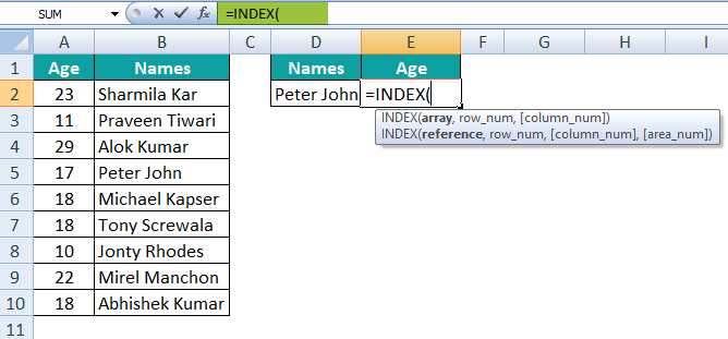
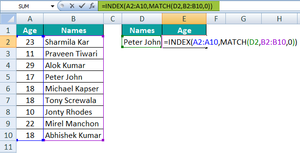
For example, below is the age data for family members:

We will try to find the age for “Peter John” using the cell reference D2.

Here, the lookup value (age) is to the right of the array, and VLOOKUP cannot fetch the data from right to left.

Hence, we have to use the INDEX MATCH function to overcome the limitation of VLOOKUP in this scenario.

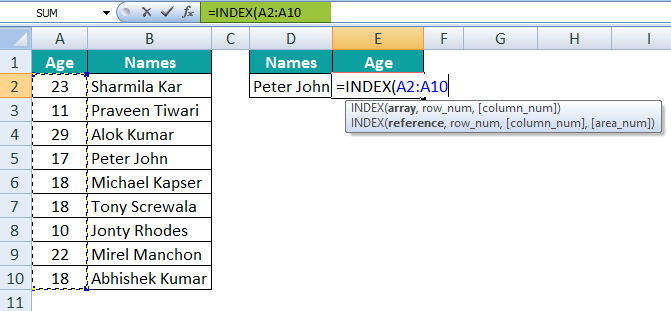
Enter the INDEX function in cell E2.
Select the age column array for the argument Array, i.e., A2:A10.
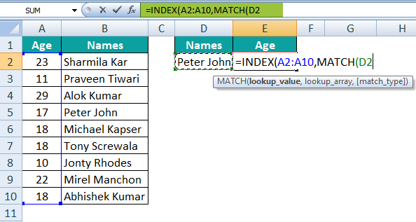
Enter the Row Number argument in the MATCH function.
For lookup value, select cell D2.
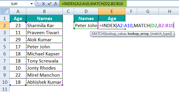
For the lookup array, select the range of cells, i.e., B2:B10.
The last argument is to select the match type. For this, we will choose the exact match, i.e., 0.
Close the bracket. It will dynamically return the result as 17, which is the age of Peter John.

Thus, we can use the MATCH formula as the supportive function for the INDEX formula as an alternative to the VLOOKUP function.

Example #2: Get Entire Row Data For The Selected Value

Here, we will understand how to get the value from the whole row. Consider the same data used in the first example.

The goal is to get the whole row data, i.e., the value for all the years for the state “DE” in cell A13.

We can apply the INDEX MATCH function in the same manner as in the above example.

For the last argument column number in the INDEX function, give the input as 0.

Hit the ‘Enter’ key after closing the bracket.

It will automatically extract the entire row value for the state “DE.”

Example #3: Get The Total Sum Of The Entire Row

With the continuation of the above function, let us find the total sum of all the years for the state “DE” in cell L3.

Apply the INDEX MATCH function as we did in the above two examples.

Do not hit the ‘Enter’ key, as we need to get the entire row sum for the state “DE.”

To do this, wrap the entire function with the SUM function, surround the whole formula with the SUM function, and hit the ‘Enter’ key.

The function will total 45,499 which is the sum of sales for all the years for the state “DE” in the cells B8:I8. The simple SUM function helps us get the result.

Important Things To Note

INDEX MATCH function in Excel combines INDEX and MATCH functions to fetch the value and position in the array.
It returns the #N/A error if the lookup value is unavailable in the lookup array.
MATCH function works as a supporting function for the INDEX function, making the combination an alternative to VLOOKUP.

Frequently Asked Questions (FAQs)

How does the INDEX MATCH function work in excel?

The INDEX MATCH function combines INDEX and MATCH functions to perform complex lookup calculations.

For instance, we can use the INDEX MATCH function to find the product category of a product. Below is the excel data of the product and its category:

We will try to fetch the product category for the product ID Mot332 by entering the formula in cell F2:

=INDEX(B2:B9,MATCH(D2,C2:C9,0))

Press the ‘Enter’ key.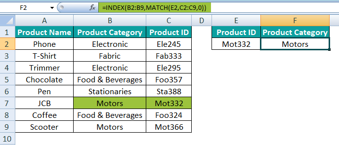

INDEX function retrieves the product category in the range B2:B9 based on the row number provided in the MATCH function for the product ID Mot332 in cell F2. The function returns the result as Motors.

Why do we use the INDEX MATCH as an alternative to VLOOKUP?

VLOOKUP has a drawback of fetching the value from left to right. If the value is to the left of the lookup value, VLOOKUP cannot work. But the INDEX MATCH function is flexible, so it does not matter how the data is organized. Hence, data structure manipulation is not required.

Which is an easy function between VLOOKUP and INDEX MATCH?

VLOOKUP is a popular and easy lookup function. However, the INDEX MATCH function is a little more complicated than VLOOKUP. In this formula, one needs to understand two different tasks and then combine them to get the result.

Which is faster between VLOOKUP and INDEX MATCH?

When the data is small, there is not much of a difference. But when the amount of data becomes larger, the INDEX MATCH function works faster than VLOOKUP.

Download Template

This article must be helpful to understand the INDEX MATCH Function in Excel, with its formula and examples. You can download the template here to use it instantly.

INDEX-MATCH-in-Excel Download

Index Match in Excel