Index Excel Function

INDEX Excel Function Definition

The INDEX Function in Excel allows the user to fetch a desired value from a particular row and/or column within one or multiple specified arrays. One can enter the formula at the desired cell in the same or different worksheet to get the desired value. The function can also fetch the single cell value, the entire row value, or the entire column value based on the table array selected.

For example, we can use the INDEX function to find the Prime Minister of a particular country based on the row number provided. The table below contains data of some countries Presidents/Prime Ministers.

We can enter the formula in any cell (D1 in this case): =INDEX(B2:B7,3).

The function searches through the table array B2:B7 and finds the value from the 3^rd row. Now, press the “Enter” key. It will give the output as “Narendra Modi” in cell D1.

INDEX Excel Function Definition

The INDEX Excel Function allows Excel users to retrieve the desired value from a certain row and/or column within one or more specified arrays at a chosen cell in the same or another worksheet.
Based on the table array selected, the function can also obtain a single cell value, a complete row value, or an entire column value.
The function has two types of syntax: array and reference.
The INDEX function in excel with MATCH is frequently used as an alternative to VLOOKUP.

INDEX() Excel Formula

The syntax of the INDEX Excel function comes in two forms, i.e., array and reference, as shown in the image below. Let us understand their arguments:

Array: The range of cells (row or column) or an array constant.
Reference: It is the area that can be a single cell range or a collection of non-adjacent cell ranges.
Row_Number: The first argument from the Array, from which we need to fetch the value of the exact row number.
[Column Num]: This is an optional argument, which we use to fetch the value from the specified row and specified column.
[Area_Num]: Again, this is an optional argument, which we can use for multiple ranges for an argument. We can provide the area number by selecting the reference from all the available ranges.

Excel VBA – All in One Courses Bundle (35+ Hours of Video Tutorials)

If you want to learn Excel and VBA professionally, then Excel VBA All in One Courses Bundle (35+ hours) is the perfect solution. Whether you’re a beginner or an experienced user, this bundle covers it all – from Basic Excel to Advanced Excel, Macros, Power Query, and VBA.

Start Learning Now

How To Use INDEX Function In Excel?

Let us look at a basic INDEX function example before we jump into some advanced examples.

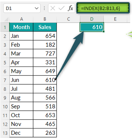
Below is the monthly sales volume of a department store.

Column A contains Months
Column B contains Sales

We need to fetch sales value for June.

Steps to Use Index Function is given below –

Enter the INDEX function in any cell (D1 in this case).
Select a range of cells, i.e., B2:B13, where we want the function to look for the sales value in June.
Since we are trying to fetch the June sales value, we will select the 6^th row of the specified array as the Row Number argument.
As we are looking at one-dimensional value, the last argument, Column Number, becomes optional here. Close the bracket and hit the “Enter” key to get the result in cell D1.

So, the result is 610, i.e., June sales value in cell B7.

Conclusion: Using INDEX function in Excel, we can get the value from the specified range of cells or arrays by entering the specific row number.

Examples

Let us have a look at a few INDEX function examples to understand it even better:

Example #1

Let us start with a two-way match with a static approach. We have created the below table in Excel, which contains employee names and the monthly bonus amount.

Now, we will try to retrieve the bonus value for the employee Ram for March.

First, we need to find the row, and then on the same row, we need to find a value from a different column.

Then we will enter the last argument of the INDEX excel function, i.e., Column Number.

Step 1: We will enter the INDEX function in the cell where we want the result.

Step 2: Now, we need to select the array. Here we have multiple values to select all the values within the array, i.e., B2:F7.

Step 3: Next, we need to enter Row Number. Since we are looking for employee Ram in the 3rd row, we will enter the row number as 3.

It is worth noting that we need to count the row or column number within the array only to get the desired result.

Step 4: Next, we will enter the Column Number argument in the INDEX function, as we are also looking for the bonus value for a specific month. Here, we are looking at the bonus amount of Ram from March, which is in column number 3.

Step 5: After entering all the arguments, close the bracket and hit the “enter” key to get the result.

INDEX excel function here fetches the bonus value, i.e., 1731, for Ram from the 3^rd row and 3^rd column of the specified array.

Similarly, if we want to look at Rameel’s bonus for May, we have to change the row number to 4 and the column number to 5, as shown in the image below.

Example #2

The above example is a static way of entering row and column numbers into the INDEX excel function, but it is a manual process.

Let us look at the dynamic entering row and column numbers in the function.

Step 1: Here, we are looking at two ways to match employee drop-down and month drop-down lists.

Step 2: We will look at the bonus amount of the employee Roja for February using the drop-down lists.

Step 3: Now, in cell I2, enter the INDEX formula.

Step 4: Select the table array, i.e., B2:E7.

Step 5: To make the formula dynamic and arrive at a row number directly, we use the INDEX function with MATCH excel function here.

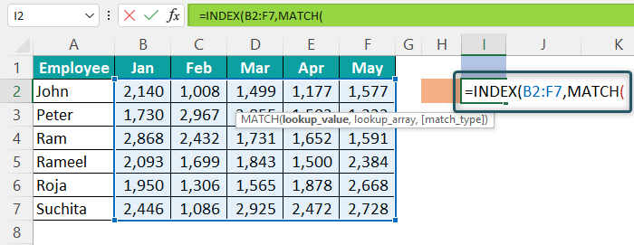
Step 6: The first argument of the MATCH function is the lookup value. We are looking to fetch the row number, i.e., employee name, in cell H2.

Step 7: Next argument is lookup array,i.e., employee list ranging from A2:A7.

Step 8: Next argument is Match Type, to find the exact match, i.e., 0.

The MATCH function will return the row number for the employee selected in cell H2.

Step 9: To arrive at the column number dynamically, we can use the MATCH function. It will fetch the column number of months selected in cell I1.

In this case, we have used the lookup value as cell I2 (month selected from the drop-down list) and lookup array as B1:F1 (this is where the month list is)

This will return the result for the selected employee and the selected month.

We can change the employee name and month from the drop-down lists. Eventually, the MATCH function will automatically return the row number for the employee selected and the column number for the month selected from the respective drop-down lists.

Example #3

We have seen two-way lookups. Next, let us look at the 3-way lookup. We compiled the below data showing employee names and their monthly bonuses.

We have 3 tables in the above image across 3 quarters. The three-way lookup will help us get the bonus amount of a specific employee from a specific month from different quarters.

Step 1: Now, let us say we want to get the bonus for the employee Peter for June.

Step 2: Enter the INDEX function and choose 3 different arrays. Select the cell references, B3:D8, F3:H8, and J3:L8. Specify the row number as 2 and the column number as 3.

Step 3: Next, we will enter the Area Number argument in the INDEX excel function. Since we have selected three different arrays, we need to specify the table from which we are trying to fetch the value. In this case, we are looking to fetch the value for Peter for June from the 2^nd table.

Enter 2 for the row, 3 for the column, and 2 for the area number.

Step 4: Close the brackets and hit the “enter” key.

Important Things To Note

INDEX function does not require a column number argument in one-dimensional lookup, i.e., only one column.
The function will return a #N/A error if the lookup value is not the same in the array.
INDEX and MATCH can be used as a nested function or alternative to the VLOOKUP formula to get the desired result.

Frequently Asked Questions (FAQs)

1. What does index function do in excel?

The INDEX function is a lookup function that allows the user to locate a certain cell value based on the row and column numbers entered.

For example, we can use the function to find who heads a particular department of a company. The Excel sheet containing records of heads of different departments is as follows: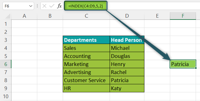

Enter the formula =INDEX(C4:D9,5,2) in cell C1. Press the “Enter” key, and the output is Patricia.

First, the INDEX function goes to the range C4:D9 and fetches the value at the intersection of the third row (row 5) and the second column of the array (column D).

2. How does the MATCH function help us make the INDEX function dynamic?

INDEX function requires row and column numbers to get the value from the desired cell. Hence, supplying the row and column numbers manually makes the task difficult.

The MATCH function dynamically returns the row and column number to the INDEX function based on the lookup value.

3. Will the INDEX function work for both horizontal and vertical datasets?

Yes, the INDEX excel function works for both horizontal and vertical data. Hence, this can be used as an alternative to both VLOOKUP and HLOOKUP with the combination of the MATCH function.

Download Template

This article must be helpful to understand the INDEX Function in Excel, with its formula and examples. You can download the template here to use it instantly.

INDEX-Function-in-Excel Download

Index Excel Function