


What Is A #DIV/0! Error In Excel?
The Division Error or the #DIV/0! Error in Excel is the error that occurs when we divide any cell value or cell reference by zero or a blank cell, or if any cell reference of a formula contains the #DIV/0 error.
For example, we will apply the #DIV/0! Error to calculate the error values as the output.

Select cell A2, enter the formula =10/0, and press “Enter”.

The result is returned as ‘#DIV/0!’ error’, as shown above.
Use this #DIV/0! Excel Error Template to follow along with the examples in this article.
Download Excel TemplateKey Takeaways
- The #DIV/0! error is caused by dividing by zero but can also be generated due to other formulas referencing cells that display the #DIV/0! error.
- It is useful because it tells that something is missing or unexpected in the data.
- It also appears when data is entered but is not yet complete or any blank cell because it is not yet available.
- If a blank cell is left in the data and division calculation is to be performed, Excel considers the blank cell value as 0, and the evaluated result will generate #DIV/0! Error.
Scenarios Of Getting “#DIV/0!” In Excel
During Excel calculations, we get “#DIV/0!” in the following scenarios,
- Dividing by Zero.
- Summing Cells.
- AVERAGE Function.
#1 – Dividing by Zero
We will perform calculations and generate the #DIV/0! Excel Error for the Dividing by Zero scenario.
In the table, the data is,
- Column A contains the Values.
- Column B contains the Output.

The procedure to get the #DIV/0! Error is as follows:
Select cell B2, enter the formula =A2/A3, and press the “Enter” key.

The result is a “#DIV/0!” error, as shown above.
#2 – Summing Cells
We will perform calculations and generate #DIV/0! Excel Error for the Summing Cells scenario.
In the table, the data is,
- Column A contains the Values.
- Column B contains the Output.

The steps to get the #DIV/0! Error are as follows:
- Step 1: Select cell B2, and enter the formula =SUM(A2:A7), to calculate the sum of the values.

- Step 2: Press the “Enter” key. The result is a “#DIV/0!” error, as shown below.

#3 – AVERAGE Function
We will perform calculations and generate #DIV/0! Excel Error for the AVERAGE Excel Function scenario.
In the table, the data is,
- Column A contains the Values.
- Column B contains the Output.

The steps to get the #DIV/0! Error are as follows:
- Step 1: Select cell B2, and enter the formula =AVERAGE(A2:A7), to calculate the average of the values.

- Step 2: Press the “Enter” key. The result is a “#DIV/0!” error, as shown below.

How To Fix “#DIV/0!” Error In Excel?
We can fix the “#DIV/0!” error in Excel using the IFERROR(), ISERROR(), and IF() functions.
#1 – Remove #DIV/0! Error Using IFERROR
We will use the IFERROR function in Excel to remove the #DIV/0! error.
In the table, the data is,
- Column A contains the Values.
- Column B contains the Output.

The steps to remove the #DIV/0! Error using the IFERROR() are as follows:
- Step 1: Select cell B2, enter the formula =SUM(A2:A3)/0, press the “Enter” key, and drag the formula from cell B2 to B3 using the fill handle. The results are “#DIV/0!” error, as shown below.

- Step 2: Let us fix the result in cell B3, to understand the difference.
Select cell B3, enter the formula =IFERROR(SUM(A2:A3)/0,“Sum is Divided by 0”), and press the “Enter” key. The result is the “Sum is Divided by 0”, as shown below.

#2 – Remove #DIV/0! Error Using IF
We will use the IF function in Excel to remove the #DIV/0! error.
In the table, the data is,
- Column A contains the Values.
- Column B contains the Output.

The steps to remove the #DIV/0! Error using the IF() are as follows:
- Step 1: Select cell D2, enter the formula =C2=B2/C2, and press the “Enter” key. We will get an error pop-up, click “OK”. The result is a “#DIV/0!” error, as shown below.

- Step 2: Let us fix the result in cell D2, to understand the difference.
Select cell D2, enter the formula =IF(C2=0,0,B2/C2), press the “Enter” key, and drag the formula from cell D2 to D3 using the fill handle. The results are “0”, and “0.8”, as shown below.

#3 – Remove #DIV/0! Error Using ISERROR
We will use the ISERROR function in Excel to remove the #DIV/0! error.
In the table, the data is,
- Column A contains the Values.
- Column B contains the Output.

The steps to remove the #DIV/0! Error using the ISERROR() are as follows:
- Step 1: Select cell B2, enter the formula =A2/A3, and press the “Enter” key. The result is a “#DIV/0!” error, as shown below.

- Step 2: Next, select cell B3, enter the formula =ISERROR(B2), and press the “Enter” key. The result is “TRUE”, as shown below.

Find All Cells With #DIV/0! Excel Error
The steps to Find All Cells With #DIV/0! Excel Errors are as follows:
- We must first open the file where we want to remove the #DIV/0! Errors. Then, press the “CTRL+F” keys, i.e., the shortcut keys to open the “Find and Replace” dialog box in Excel.

- Click on the “Options” button, which shows additional options.

- In the ‘Find what:’ box, type #DIV/0!

- From the ‘Within’ drop-down with the Sheet or Workbook options, select the “Sheet” option.

- From the ‘Look in’ drop-down, select the ‘Values’ option.

- Click on “Find All”, which will find all the cells that have the #DIV/0! error, as shown below.

Important Things To Note
- We get a #DIV/0! error in the AVERAGE function when the dataset does not have any numerical value.
- The #DIV/0! error occurs in the SUM excel function when the selected cell range has one or more of the cell values as the #DIV/0! value in it.
- We can avoid getting a #DIV/0! Error by making sure that a division calculation doesn’t have the divisor as 0 or the excel cell reference for the divisor is not a blank cell or 0.
Frequently Asked Questions (FAQs)
Let us consider an example where we get a #DIV/0! Error due to blank cells.
We will first divide the values, and generate the #DIV/0! Excel Error when the reference cell is passed is blank.
In the table, the data is,
• Column A & B contains the Values.
• Row 3 contains the Output.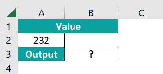
The procedure to get the #DIV/0! Error with a blank cell is,
Select cell B3, enter the formula =A2/B2, and press the “Enter” key.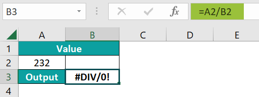
The result is a “#DIV/0!” error, as shown above.
The #DIV/0! in Excel means that there is a division error in the formula or the cell reference, such as a number divided by zero, or the dataset has a blank cell, or the result of the formula is zero, which is the number getting divided.
We can display a Zero instead of #DIV/0! Error as follows:
First, create a data table, as shown below.
Next, choose cell B3 → select the “Formulas” tab → go to the “Function Library” group → click the “Insert Function” option on the far left, as shown below.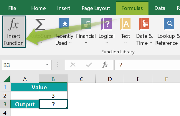
The “Insert Function” window appears. In the “select a category:” drop-down, select the “Logical” option, as shown below.
Now, the options change in the “Select a function:” group, then select the IF function, and close “OK”, as shown below.
Once we click “OK” in the “Insert Function” window, the Function Arguments window appears.
Enter in the Logical_test field as A2=0, the Value_if_true field blank, the Value_if_false field as B2/A2, and click “OK”, as shown below.
So the complete formula will be =IF(A2=0,,B2/A2). We will get the result ‘0’, as shown below.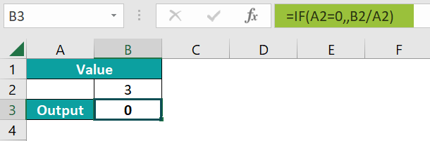
Use this #DIV/0! Excel Error Template to follow along with the examples in this article.
Download Excel TemplateRecommended Articles
Continue with these related resources when you want the next practical step in this topic.
- Errors In Excel
- Excel Troubleshooting
- Excel Formula Not Working
- Circular Reference in Excel
- IFERROR In Excel
Explore the full Excel Errors and Troubleshooting guide or browse Excel Resources.